If planning constrains housing supply, how does it do it?

I’ve long puzzled over the exact mechanism by which planning regulations are supposed to constrain the rate of new housing supply. Sure, they constrain the locations at which different types and densities of uses can occur. That’s their purpose.

But density (dwellings per land area) and the rate of supply (new dwellings per period across all sites in a region) are very different.

It seems logical to me that landowners maximise their economic returns from two choosing

1. a density of development that maximises the residual (i.e. their revenue minus the cost of development), and
2. a rate of sales (and hence development) per period of time.

It is not at all clear that if more dwellings can be built on one site that this changes the optimal rate of sales per period for that site.

It is also the case that only landowners can choose to make planning applications, and that a huge majority of approvals are for projects that exceed coded density limits. We have a property market after all.

What I am puzzled about is that when someone claims that planning reduces housing supply, what sort of counterfactual pattern of supply do they have in mind?

...

Read the rest of this post at my new substack page and please subscribe there to get new posts to your email.

My COVID story - Part 1

March 2020 — People lose their minds

My first ever public comment about COVID was this. I was both prescient and wrong.

Everyone has lost their shit about coronavirus as if lives lost this way are worth orders of magnitude more than lives lost any other way. In two to three weeks time the reality will set in that there are real costs of locking down society that can be measured both in value of resources wasted and in blood. All perspective has been lost at present.

If only I’d written years instead of weeks, then it would have been spot on.

As someone who has thought about health policy, well-being, and trade-offs for many years, my first reaction to the media coverage of COVID and the mystery China virus was to ask the following question: What is the normal number of deaths in a city the size of Wuhan? Without this context, all the media coverage made no sense. A city with 12 million people can expect about 96,000 deaths a year. That’s 264 a day.

So when I read headlines like “Death toll rises to 600” and that smoke from crematoriums working overtime was filling the city, I had a reasonable baseline from which to sniff out nonsense. The numbers mattered then and they still matter now.

If you search online for news articles of COVID or coronavirus deaths from February 2020 you will see just how small the death numbers are and how crazed and fearful the reporting was. Some of the reporting just had made-up figures, with orders of magnitude differences from one article to the next. No one really cared.

Even at this early stage, the lack of deadliness of the virus was becoming clear for those who wanted to find out. The case fatality rate was likely to be sub 0.7%, even with relatively limited testing (i.e. 0.7% of known cases, not all cases). Clearly, this implied that early estimates were hugely biased because infections were far more widespread than initially assumed.   

The Diamond Princess cruise ship had 3,711 people on board and had 14 deaths.  On this cruise, 0.37% of people died over a two month period. Is that good or bad?

We know that background mortality is about 0.8%. So every two months you can expect 0.13% of people to die. But this is across the whole age distribution. Even a small skew towards the elderly massively increases this number. For example, in your 80s you have a one in twenty chance of dying each year on average. In your 90s, a one in five chance.

The age distribution of the Diamond Princess was super high, so 0.37% of people dying within two months is totally within the normal range.

We knew this in March 2020.

Image source: https://wattsupwiththat.com/2020/03/16/diamond-princess-mysteries/

We already knew then from the Italian outbreak that the average age of COVID deaths was higher than deaths from all other causes combined.

Taking all this information together was pretty encouraging. This is why herd immunity was thought to be simply a matter of months away. Flatten the curve for two weeks, then a month or two later the whole thing would be over. No one expected to be having masks, border closures, vaccine mandates and passports for two years.

With markets crashing I took the opportunity to put forward some ideas about macro-stabilisation policy, such as having a public agency take equity stakes in companies that wanted bail-out money and buying up housing developments in distress to smooth construction cycles and add to public housing stocks.

Of course, none were taken up. But looking back, they were much more sensible than what we got with a JobKeeper giveaway, a Cashflow Boost, that cost hundreds of millions and resulted in a net upwards redistribution of wealth.

Read the rest of this post at my new substack page and please subscribe there to get new posts to your email.

New metrics to show the value of delaying housing supply

*This article is based on a submission to the Housing Supply Inquiry that I contributed to for Prosper Australia.

This neglected economic puzzle has become a heated policy debate. Rapidly rising dwelling prices globally have grabbed the attention of policy makers. Many have subsequently targeted planning and zoning as areas for housing reform. Australia, New Zealand, the United Kingdom and various states in the United States, are conducting new reviews into planning, housing supply, and prices.

Unfortunately, most analysis of housing supply conflates density (dwellings per unit of land) and the rate of new housing supply (new dwellings per period of time across all sites). This is because the time dimension of the investment decision facing a landowner is typically ignored in the economic analysis of housing supply.

But the optimal inter-temporal choice of landowners is hugely important for understanding the rate of new housing investment in property markets. Just as there is an optimal density of development that maximises the value of the site, there is also an optimal rate of sales of new dwellings per period that maximises the value of the site.

Across all candidate development sites in a region, the rate of new housing development (new dwellings per period of time) is known as the market absorption rate or build-out rate. Regardless of planning or zoning, this rate is the result of many landowners making individually-optimal choices about when and how fast to develop. 

The economic logic behind the market absorption rate is described in Murray (2021). Some key elements of it are important to clarify. Owners of the property where a new home can be built already possess an asset on their balance sheet worth exactly the market value of the land. Developing that land with a new dwelling is a balance sheet reallocation. If developed for immediate sale, the property owner is swapping an undeveloped site asset for a cash asset. If developed for rental, the owner has swapped an undeveloped land and cash asset (to fund construction) for a dwelling asset. 

Whether these asset swaps are economically viable depends on the relative returns to each. Only in a market where demand is rising does it make sense to increase the rate at which undeveloped land assets are swapped for cash assets. When market demand is falling and very “thin” (few buyers at current prices), it makes sense to slow the rate of new housing development. Other factors like interest rates (the return on cash after sale), taxes on land ownership (that reduce the return to retaining ownership of undeveloped land), and the ability to vary the density of development in the future (a flexible planning system can make delay more profitable by allowing higher density in the future, increase the return to delay), all have effects on this rate. 

One interesting problem for this new type of analysis is demonstrating how economically important the payoff to delaying new housing development is for property owners. To address this, I am proposing here some new metrics that can be applied to housing developments to demonstrate the degree to which varying the rate of sales in response to market conditions increases the total economic returns from developing a site. These metrics demonstrate that independent of any planning controls on density, there is a “speed limit” on the supply of new housing in the form of the market absorption rate.

Development Rate Ratio (DRR)

How fast did the subdivision develop compared to how fast it could have if the maximum observed rate of sales was sustained?

Housing developers often argue that new housing is being built as fast as the planning system allows. Indeed, quite a deal of economic analysis also makes this assumption. However, once a subdivision or apartment building is approved by the planning system, the private choices of the developer determine how fast the approved new housing is developed. This includes how fast they sell, which is the key limiting factor of the build-to-order model of new housing production. 

To demonstrate the degree to which these private choices limit the potential rate of new housing supply I proposed looking at the Development Rate Ratio (DRR). 

The DRR shows the average speed of development as a ratio of the maximum speed, using the average monthly rate in the fastest three-month window. A lower number indicates that the new housing development proceeded more slowly than was demonstrated to be possible.

Development Rate Variability (DRV)

A second metric is Development Rate Variability (DRV). DRV is the ratio of the fastest speed of monthly sales to the slowest monthly sales during a development. This shows how sensitive to market conditions the choice of sales can be. A higher DRV shows how much the private choices of housing developers change the rate of new housing supply. 

It may be argued that it is impossible to sell fast in a depressed market. But this is only true if prices are held constant. The very heart of the housing supply debate is whether planning changes create conditions for private housing developers to build faster at lower prices.

These two new metrics can help paint a picture of the variation in the market absorption rate due to the private choices of landowners. To complement these metrics, we also create new metrics of the economic returns available in housing development from varying the rate of supply in response to market conditions. 

Delay Premium (DP)

What is the economic gain from varying the rate of supply of new housing to “meet the market”?

To answer this question a sensible counterfactual must be established. The counterfactual implied in most economic analyses of housing is that housing is supplied once the market price gets above the feasible price for development. In other words, housing developers fix the price of all housing (or land lots) at the beginning of the project (a fixed point in time) then vary only the speed of sales to match market demand at that initial feasible price. 

The dynamic approach recognises an economic return to varying both the rate of supply and the price. This is then the difference in revenue between the following two approaches.

1. Setting a price at the beginning of the project and selling all dwellings or housing lots at that price until the project is completed
2. Varying both the rate of supply and price to maximise profits from the project. 

A metric that identifies the economic gains to delay is the Delay Premium (DP). The DP is the share of total revenue that was made by varying price as well as quantity (ignoring discounting) and is calculated as follows.

Two parts of this equation need some explanation. First, when applied to detached housing subdivisions the total revenue is for land only, not for homes. This is because the additional gain from building the home comes with added construction costs leaving the land value as the net income. Second, the reason for including the minimum land price rather than the initial price is because the lowest price in the sequence of sales indicates the minimum willingness to sell. 

A higher DP means that a larger share of the total revenue came from actively varying both price and quantity during the selling period. 

Available Delay Premium (ADP)

Another metric that shows the economic gains to delay is the Available Delay Premium (ADP). It measures the maximum difference in sales price over the life of a project (the peak price per sqm that often occurs at the end of a project and the lowest sale price that usually occurs near at the beginning) multiplied by the total sold land area as a proportion of actual revenue. This metric indicates a theoretical maximum degree to which revenue could have varied (as a proportion of actual revenue) if all sales were made at the highest price compared to all sales being made at the lowest price.  

The interpretation of the ADP is to show how important choosing the timing of sales can be to the final returns of a project. A higher ADP indicates that varying sales rates due to changes in demand, and hence price, will have a higher economic payoff.

Applying these metrics

Jordan Springs is a 900-hectare residential subdivision located in Penrith (53km west of Sydney’s CBD) and was approved for development in 2009 with the first residents moving in during 2011. 

By 2012 the development was owned by Lendlease, which published in its annual report that year that the area would ultimately provide over 2,000 detached dwellings and 200 apartment dwellings, with an expected 10-year development timeline. The subdivision masterplan is below. 

Unfortunately, data on land and house sales in this subdivision is only available to me at the moment from 1st October 2015 to 8th October 2021, a period over which there were an estimated 2,131 new land lot or dwelling sales.

Summary of absorption rate metrics

The four absorption rate metrics for the available data on this large subdivision project are summarised in the table below. 

In this data, total revenue was around $1 billion. The 0.13 DP represents about $137 million of value that was gained by varying prices during the project rather than setting the minimum profitable price and selling all lots at that price. The difference in revenue between selling all lots at the lowest per square metre price and the highest price was $310 million. These figures also provide insight into the variability and risk involved in land and housing development. 

Further analysis and detail

It is also worth looking at the variation in sales and prices over the available data for the Jordan Springs project. 

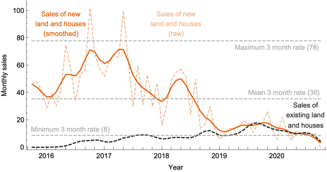
The chart below shows the smoothed monthly rate of land and house sales for new dwellings (orange), alongside the repeat sales (dashed black) over time. Minimum, maximum and mean sales rates are marked (which are used to generate the DRR and DRV metrics). Notice that in the quiet housing market of 2019 that sales were much slower than in the busy 2016-17 market period. 

The next chart below shows the land price per square metre observed in the sales data over the same time period, with maximum, minimum and mean prices market (which inform the DP and ADP metrics). During this five year window, land prices varied by around 30% (the ADP metric) but had noticeable peaks and troughs that coincided with macroeconomic conditions. 

Finally, we can look at the relationship between price growth and the rate of supply in the final chart below. Although these data points do not generate a statistically significant relationship, visual inspection shows clearly that periods observing price growth also saw faster new supply, especially in earlier development stages during 2016-18, as expected if the developer is optimising sales rates and price to maximise their revenue (as predicted by the logic of the market absorption rate). 

The enormous variation in the rate of supply in large projects such as Jordan Springs, with thousands of approved dwellings, is a clear indication of macroeconomic and market conditions being the main determinant of the rate of new housing supply.