The puzzle of high home prices and vacant homes

One pattern that stands out in the property market is that although homes prices are at all-time highs, so too is the proportion of vacant dwellings. This is a puzzle. How can it be the case that when housing is in high demand it is also rational to keep more housing vacant?

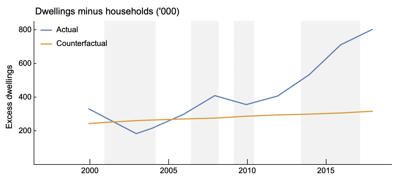
Australian data shows that the number of residential dwellings has grown faster than the number of households for the past decade, indicating a substantial rise in the proportion of empty homes. This phenomenon has been a broad one, experienced in cities such as Sydney, Vancouver, and Toronto. Here are some of my previous thoughts on the topic.

The resolution to this puzzle is as follows. Housing is an asset, and in asset markets there is a trade-off between liquidity and returns. A vacant home is a more liquid asset than an occupied home. Timing a sale is easier, the sale is faster, and it is likely to result in a higher price when vacant. When capital gains are a large proportion of the total return, and capturing this return requires timing the market because of price variability, the value to liquidity from vacancy can be high.

In short, when yields are low and prices high and variable, the benefits to vacancy are high.

Here’s an example. In Scenarios A and B the total asset return to housing is 10%. But in Scenario A the price is high and yields are low. Here, leaving the property vacant forgoes only a quarter of the total return from the asset. If prices are variable in this Scenario, then timing a sale becomes an important factor for earning the capital gains. Hence, the liquidity from vacancy has a large benefit.

	Return	Cap. gains	Rent
Scenario A	10%	7.5%	2.5%
Scenario B	10%	2.5%	7.5%

In Scenario B the price is low, as the rental yield is 7.5% of the price. Capital gains are also low at 2.5%. In this low price, low capital gain, scenario, keeping the property vacant requires giving up three-quarters of the total return. The benefits from doing so are limited since capital gains are low, and hence less variable.

So there is an economic logic behind the puzzle of high prices and high vacancy, and it stems from the fact that housing is an asset as well as a consumption good. But there is also a criminal logic. Much of the vacant housing in Australia (and probably Canada and a few other locations) is due to money laundering. There are no checks on the source of finance for home purchases and no checks on who the ultimate beneficiaries are in the ownership structure. You can buy a home in a trust or company name, and the identity of the trustees and the company owners need not be disclosed. If you then also do not earn rental income, the corporate structure is protected from scrutiny by tax authorities. Housing is a great way to hide ill-gotten gains.

The criminal logic and economic logic are closely aligned. When most of the return to housing comes from capital gains it makes housing a more attractive place to hide money as three-quarters of the total return can still be had. But when most of the return comes from rent it is much less attractive — and it may require corporate disclosure due to local incomes warranting taxation.

Finally, some new data
On another note, new data from the Australian Bureau of Statistics came out recently, filling one of the holes in the housing data landscape — the share of lending to investors that is directed towards purchasing or building new homes.

This data helps to answer questions about the economic value of new credit in the economy, the real economic effects of monetary policy, and more. In standard economic thinking, low interest rates make borrowing to invest in new buildings and equipment more viable. Because standard economic models do not include secondary markets, the effect on the trade of existing assets is mostly ignored. Yet we can see that the majority of home purchases are simply trades of existing housing, and hence are a key mechanism through which low interest rates mostly cause higher prices without having much effect on new construction.

As you can see in those few months of investor data,  investor lending is not substantially more biased toward new housing than lending for owner-occupiers. For investors, 24% of loans have been for new housing in the past few months, just as 24% of loans to owner-occupiers have been.

The main difference seems to be that the typical existing home bought by owner-occupiers is more expensive than the typical new home, whereas for investors the mean value of lending to both is the same. 

Rent control is totally normal price-cap regulation

Bernie Sanders has smashed the Overton window. Rent control is going global.

Unfortunately, this means that the economics 101 brigade has come out in force to smugly Vox-splain their incorrect model of rent control and housing market dynamics.

The Onion’s Vox parody is so spot on I can’t stop laughing pic.twitter.com/Q9oQKFr46P

— 𝐂𝐚𝐫𝐥𝐨𝐬 (@ChuckEChaves) September 15, 2019

Regulating housing rents makes economic sense because homes are attached to land monopolies. Monopolies are inefficient, and regulations can improve outcomes. The two classic regulations are 1) a tax on monopoly super-profits, which is common for mineral and energy resources, and 2) a price cap, which is usually applied to network infrastructure, like rail, electricity, and water. If price caps sound to you a bit like rent control, then you would be spot on. They are rent control.

Rent control is not weird or unusual for regulating monopolies. The weird thing is that land is no longer considered a form of monopoly.

Let me explain how these two classic regulations would work in housing markets to socialise monopoly profits from housing locations.

A super-profits tax would work like this. When a new home is constructed, the owner would be able to seek the market rent. That first year’s market rent would become the regulated price that would attach to that home in a rental database. The home would still be allocated in the rental market using open market prices. But any gap between the market price and the regulated price would be 100% taxed. This is shown in the figure below.

If the market price fell below the regulated price for some reason, that loss would accumulate as a credit against future tax obligations when the market price increased again.

With a super-profits tax system housing resources, including new construction, are always allocated by market prices.

Since the financial crisis, rents have increased by roughly 25% in the United States. A quick guess-timate suggests that around a trillion dollars of rents are paid in the US each year. Had such a tax been implemented ten years ago it would now raise about $250 billion a year with no efficiency loss. In Australia, total housing rents have increased from around $30 billion to $45 billion in that period, meaning a housing super-profits tax would now raise around $10 billion per year (after adjusting for the increased housing stock).

The second way to regulate the land monopoly in the housing market is with price caps (rent controls). Here, the sitting tenant is protected from price increases that are not the result of additional housing investment or renovation but arise due to the favourable location-monopoly of the owner.

As before, market prices match tenants to housing and provide incentives for new construction. However, a sitting tenant is protected from price increases that arise from the location-monopoly. This only works if their tenure is secure, and they cannot be evicted as a way to change the rental price back to the market price.

The image below shows how the gap between market price and rent-controlled prices is a transfer to sitting tenants. If market prices fall below the regulated price, the tenant can have the option to renegotiate or move to pay the lower market price. Again letting markets decide resource allocations. It is only in periods of rapid price growth that sitting tenants are protected.

On balance, this type of regulation transfers some monopoly super-profits to tenants in the short-term but gives them back to owners as tenants relocate and homes are again allocated by market prices.

Either system of regulations will socialise some of the monopoly rents in housing markets. In fact, it is widely acknowledged that a reduction in volatility of returns can accelerate new housing investment. Recent studies also show that owners of older housing choose to accelerate redevelopment into more dense housing if their rents are regulated.

Both regulations are common in other monopolistic sectors of the economy. The main issue is that these regulations will transfer billions of dollars of value away from landlords, and landlords won’t like it. And the economic 101 brigade will always find a way to argue that policies to help the poor are bad for them.

Housing subsidy and UBI confusion

When the Australia government introduced a cash grant for first home buyers, the aggregate effect was to increase home prices by roughly the amount of the grant, quickly negating its effect on affordability.

This observation has led many people to mistakenly believe that giving cash grants in any form will pass through one-to-one into higher home prices (or rents). In discussions of all types of welfare—from UBI, to traditional welfare payments—this error comes up.

The error comes about because people fail to see that when given a choice, people spread their extra buying power across all the different types of goods they consume. An income subsidy is not the same as a subsidy for a particular type of expenditure.

Economists have been studying the way spending patterns vary with income for over 150 years. Ernst Engel noticed in 1857 that as incomes rise, households spend a lower proportion of their income on necessities like food. This observation became known as Engel’s Law, and the income-spending relationships for different goods became known as Engel Curves.

Housing, like food, is a necessity. As such, the share of income spent on housing usually falls as incomes grow. The Australian data shows that even for private renters—where one would expect competition from higher-income renters to bid up housing rents—the share of income spent on rent falls from nearly 50% of gross income for the lowest income quintile households to just 13% for the highest-income households.

This data might seem to imply that it is possible for up to 50% of a cash welfare payment to “pass through” to landlords for low-income households. But remember, this is not the marginal amount that would come out of extra income. Because the share of spending on housing falls as income rises, the spending on housing out of the extra income must be far lower than the average. In fact, across income quintiles in Australia, the marginal additional spending on housing per dollar of additional income sits tightly in the 5-7c range. It may be possible that long-run adjustments mean that more than this marginal amount is spent on housing out of extra income, but it will always be less than the average amount.

The story is rather different, however, if welfare payments are tied to a particular type of spending. This even more important in the case of housing, where the total stock changes extremely slowly and where landowners have monopolistic incentives to prefer price gains over investing in additional supply.

An example is if everyone received a fixed $1000 per month that could only be spent on housing. Because this money cannot be spread across the consumption basket, people would soon learn that they are best off using it to bid up the rent to access their preferred housing location. The macroeconomic reality is that this additional buying power will chase roughly the same number of dwellings, increasing their price.

The difference between a “general income subsidy” and a “housing expenditure subsidy” can be shown using Engel curves. The chart below shows three Engel curves for a household, with the orange representing housing. Blue represents other normal goods, where expenditure rises with income, but a bit faster than for necessities (as per Engel’s Law). The green curve is an inferior good. Household spend less on these goods after their income reaches a certain level.

A “general income subsidy” shifts the household up to a higher income level, and they spend more on all the types of goods in their consumption basket. The effect on housing expenditure is relatively small, as expected by our previous 5-7% assessment of marginal housing expenditure.

The next chart shows the effect of a “housing expenditure subsidy”. The total income of the household is unchanged. They are only able to direct the subsidy towards their housing expenditure. Here, the effect will be to boost buyer competition for scarce housing locations and increase home rents (or prices). This was the case with the first home buyers grant.

Though it is tempting to see them as quite similar, subsidising household incomes and subsidising a particular type of expenditure have rather different economic effects. 

Microeconomic success, macroeconomic failure

When I teach macroeconomics, I use a dog and bone analogy to demonstrate that the macro-economy is not equivalent to just “adding up” the micro.

Let’s see the analogy in action.

In the dog and bone economy, ten dogs repeatedly try to find nine bones buried in the yard. Each round, at least one dog misses out. We think that this outcome is undesirable— we can’t have an economy with over 10% dog “bone poverty” and perpetual “dog unemployment”!

Some astute dog economists notice that dogs that miss out on a bone are usually a little slower, or have some other traits that make them relatively poor performers. They reason that there is a “skills mismatch” that, if corrected, could solve the macro-economic problems in the dog economy.

These economists go the extra mile and conduct some randomised controlled trials on interventions that seem promising.

1. Give the dogs that miss out a head start
2. Provide the dogs that miss out advice about where to find the bones
3. Train the dogs that miss out to sniff out bones better

After trialling each of these interventions, the results come in. They are astounding!

In each policy experiment, dogs that missed out on finding a bone 75% of the time in the control group only missed out 5% of the time in the treatment group.

The researchers responded to media enquiries about their results. “This is the largest effect I’ve ever seen in a social science intervention,” they said.

If it can be replicated at scale, the experimenters may have hit on a powerful new tool for dismantling bone poverty in the dog economy. Policymakers are now looking to invest in expanding these programs in dog parks across the country.

I don’t know about you, but it always helps me to understand what is really going on when we talk in the abstract. In the dog economy, it is clear that regardless of the microeconomic success of these interventions, there is still going to be “dog poverty” and “dog unemployment” because of the macroeconomic conditions. There are always nine bones and ten dogs. At least one dog still misses out and experiences “dog poverty”.

Helping someone jump the queue for access to scarce resources is obviously going to help that individual. But it can’t help everyone in the queue.

And yet, these microeconomic “queue-jumping” policies are politically attractive. Job training is widely thought to be an important tool for solving unemployment. But if the unemployed are competing over scarce jobs, then job training can only change the preferred ordering of candidates.

A recently popular policy in this vein has been “intensive housing counselling”. This involves lobbying landlords on behalf of housing voucher tenants and advising these tenants to move to “high opportunity areas”. Not surprisingly, these tenants took up the professional advice and assistance given to them.

As one tenant noted, after deciding where they would like to move, the housing counsellors “pretty much took care of the rest. I gave them my information, they gave my information to the leasing office, they applied for me, and they helped with the first month’s rent and the renter’s insurance for a year.”

Making renting and finding a home easier is great. I’m not going to argue against that.

But what puzzles me is this. Like the nine dogs and ten bones, not everyone in a “low opportunity area” can move to a “high opportunity area”. And in fact, as people start to move out of these “low opportunity areas” those areas will have even fewer economic opportunities for residents that ultimately move into them! The policy can’t “add up” to the macro, despite its success at the micro-level.

So what sort of policies do work at a macro level?

In the dog economy, the thing that works is to compress the “bone distribution”—take the nine bones, cut off one-tenth of each bone, and let the ten dogs access 9/10ths of a bone each. Alternatively, have a handler keep some bones in reserve to share amongst the dogs that miss out. Macroeconomic success requires a mechanism that changes the nature of the game itself, rather than the individual behaviour within it.

Two problems with opportunity cost

If there is one idea that defines economics, it is opportunity cost. Unfortunately, muddled thinking about this idea means that across the economics discipline it is applied rather inconsistently. Economists often use the word to mean whatever they want it to mean. 

In its most basic form, opportunity cost just means your next best alternative use of resources. What opportunity did you forgo to undertake this action instead of an alternative? But it gets much more difficult to translate this idea consistently into more detailed economic theories.

I want to highlight two big inconsistencies with the use of opportunity cost in economics. To do that I want to start with a question that triggered a mini-controversy in the discipline a few years back when it was revealed that economists did worse than chance in answering a multiple-choice textbook question about opportunity cost.

The question was:

You won a free ticket to see an Eric Clapton concert (which has no resale value). Bob Dylan is performing on the same night and is your next‐best alternative activity. Tickets to see Dylan cost $40. On any given day, you would be willing to pay up to $50 to see Dylan. There are no other costs of seeing either performer.
What is the opportunity cost of seeing Eric Clapton? A. 0, B. 10, C. 40, D. 50.

According to the textbooks, the answer is B.

There are two mistakes here.

Comparison with different costs

First, the two given alternatives have different resource costs. If you see Dylan you have $40 less to spend. Therefore, a clean comparison of opportunity costs requires us to compare these alternatives

A. See Clapton for free.
B. See Dylan that night and have $40 less to spend.

If we don’t account for the full costs of each alternative, we end up with ridiculous scenarios, like comparing the profit from investing $1m with the profit from investing $1k. It makes no sense when we abstract into raw financial terms, and it makes no sense here either.

Strictly speaking, the correct answer is $10 minus the net benefit from my next best use of $40. But then again, maybe I don't know what opportunity cost is either!

Alternative options are not discrete

Another problem with opportunity cost is that, in reality, there is a continuum of alternatives to any action. The next best option to Alternative A is usually doing Alternative A but cutting some corners slightly. In this case, if seeing the Clapton concert is Alternative A, then seeing Clapton and going to the bathroom when your favourite song is played might be a “next best” alternative.

We could, if we want, break out any of the discrete alternative actions into an infinite array of alternatives. Each of those could be broken out again until we have a continuum.

If we zoom in on this continuum, then the opportunity cost is always equal to best Alternative, and even the opportunity cost of the best Alternative is itself.

This point is important. If, for example, we think that supply curves include opportunity costs of resources, then economic profits are always zero or below by definition.

In a topic I study, property markets, this is also important. Many people think that the second-best alternative use of land sets the price. For example, in regard to the price of land for housing:

…in the absence of any restrictions on supply, the price of raw land on the fringes should be tied reasonably closely to its value in alternative uses, such as agriculture.

Why is agriculture the next best alternative to housing? Surely there are multiple residential subdivision options that are alternatives, and some will be better than others.

Property valuers (appraisers) are clear that the value of property rights comes from its highest and best use, but for some reason many economists think they know better. Valuers test out the various legal options for land use to determine which one provides the highest value to land, and it is this use that determines its value.

The opportunity cost logic, in this case, becomes more absurd when we think about the case where there are three possible legal uses of land—say agriculture, industrial, and residential (in order of value). If the second-best alternative sets the price, then you can make the land cheaper by regulating against the second-best use of industrial development, making agricultural use the second-best alternative and decreasing land prices for housing.

And I haven't even considered the case when there is only one allowable use of land. Doesn't this make the second-best use to do nothing, therefore bringing the land price to zero?

Like many seemingly insightful economic ideas opportunity cost is less powerful than it appears and often confuses more than it clarifies. 

NOTE: Here are some recent articles that follow up on the original survey question that show just how varied the interpretations of opportunity cost can be.

The bathtub analogy of housing supply

Many people hold the view that rezoning land to allow higher density residential uses on each plot will accelerate the rate of city housing development.

I think this is wrong.

The main reason I think this is because there are a finite number of new buyers per period, and residential developers are not in the business of competing with themselves on price. No sane developer floods the market with new housing just because the regulations are changed to allow them to build 100, rather than 50, homes on their lot. In fact, they might just build at the same rate on that lot for twice as long before moving to the next location.

A key confusion in housing supply and zoning discussions is that density limits per lot are interpreted incorrectly as a constraint the rate of new housing supply per period. New homes per lot is not the variable of interest in city housing supply. New homes per year across all lots in a city is the critical variable.

Zoning constrains the location of different densities of housing, but not the total rate of supply across all lots in a city. [1]

In the past, I have tried to dispel some of the key problems with the standard static economic models that conflate the allowable density per lot with the rate of supply. This is what I said then about these models 

The only problem is this. When you convert the model to English you realise it has little basis in reality. The only real pattern that is consistent with the model is that higher buildings are near the city centre. But I could come up with a million other models that are consistent with that pattern.

One of the main flaws in the AMM model is that there is no possibility for development of sites within the city into new buildings. Every site is already used at its optimal level. There are no vacant sites or sites with old buildings ready for knock-down and reuse. There is no development industry. There are no landowners.

Also because of the comparative-static nature of how the model is used, every time there is a marginal change in any of the parameters of the model — a new person moves to the city, the rental price of the second best land use increases, or the efficiency of construction methods change — the whole city is wiped clean of homes and buildings. The single social planner who controls everything in the city then dictates that the whole city will be rebuilt with a new optimal allocation of housing and commercial buildings under new conditions, and this whole new stock of buildings rebuilt in an instant to that new specification. 

In that blogpost I introduced some new ideas about how to conceptualise regulatory constraints using this diagram.

I want to now offer a simple “bathtub” analogy that demonstrates why our thinking about housing supply and zoning is often misguided. 

Imagine a city region is like a bathtub. The limit on total development, if every location was used to its highest-value use, is the depth of the tub. This is affected by geographic, regulatory, and economic constraints. The water level is the current total stock of housing across the city. Lastly, the dripping water from the tap is how fast new development is occurring across the total city to increase the total stock of housing. 


The question is, what part of this bathtub situation would you address with policy changes to increase the depth of the water? The depth of the bathtub, or the rate of water flow from the tap?

Changing the depth of the tub is a bit like rezoning the whole city for higher density. It seems intuitively like a good idea, but if the city is nowhere near its bathtub capacity, what mechanism is there for this to affect the rate at which the tub gets filled?

The more effective approach is the look at the tap, and the rate at which new housing is developed. This can involve a few things, like making it more costly for landowners to delay converting land into higher-value residential uses. Or, it can mean redirecting credit flows into new, rather than existing housing, to encourage new supply. Regardless, when you start to look at the tap you see that the key variable that needs to be tweaked by policy are the dynamic incentives of landowners—delaying, or slowing, development needs to be made relatively more costly.

However, when you start to focus on the rate of supply you realise that the challenge of tackling price booms with supply is far from as simple as they seem. To even maintain the current drip feed rate of new housing requires a substantial portion of the workforce, and it doesn’t change the total stock very much (just a couple of per cent per year).

In Australia, for example, our housing tap drips at a rate that is around 2% of the total stock, and it requires something like 5-7% of the workforce to build at this rate (and more in some cities with high rates of housing construction).

To have a meaningful effect on the total stock housing, and therefore the price, requires an economically significant long-term construction boom. For example, increasing the rate of new supply by 50% for a decade—employing more than 7.5% of the total workforce instead of about 5%—will increase the total stock by just 9.8%. By any metric, this will have a price effect in the range of 5-15%. The point being, the large changes in the rate of supply have small effects on the total stock and these require a large share of economic resources shifted away from current uses and towards housing construction over a long period, particularly in boom cities.

Now, I am totally supportive of a sustained effort to build more housing to provide more options for households. But I am against pretending that rezoning means that developers voluntarily, and dramatically, increase the rate that they supply new housing to such a degree that they subsume a substantial portion of the workforce while at the same time reducing the price of the asset that earns them a living.

To change the rate of supply requires changing the dynamic incentives of landowners by making it relatively more costly to delay new housing development. This cost to delay means that bringing forward development, even if a lower price must be accepted, becomes viable. These types of changes will be labelled as punitive by landowners, but that’s how you know they are effective—it forces them to build housing when they prefer not to.

Finally, we can always create non-market housing institutions that build new housing regardless of market conditions, allowing this organisation to actually build at a rate that will depress prices, or offer housing to residents at below market prices.

With a bit of luck I hope that in future conversations about housing supply and zoning that the rate of new housing supply per period across all lots is no longer conflated with the allowable density of housing per lot.

fn. [1] I do note that some cities may very well have planning regulations that are so poorly designed that they do in fact constrain the rate of supply.

Update: Total employment in housing construction reduced to remove the engineering construction workforce.

Rising home prices reduce the willingness to supply homes

TL;DR

There is a major flaw in the idea that high prices stimulate more housing supply. It is that high price growth itself decreases the willingness of landowners to supply land for housing. 

Supply and demand (AKA Static Production Theory, or SPT)

“If we want to create widespread affordability, so that anyone can walk into a real estate office and rent something reasonable, then we must confront the laws of supply and demand.”

So says Ed Glaeser, the highest profile urban economist of this century. He has forged a career from restating this conventional wisdom, and now major national governments and institutions, including the Reserve Bank of Australia, generally prescribe to this view.

Underlying this view is a single-period, asset-free, model of the world where higher prices induce more supply of housing. New housing is a simple production process that combines land and construction inputs. As long as the price of a home exceeds the input costs of land and construction, each of which is determined by their own independent markets, profit maximisation says that these homes will be immediately produced.

In the notation, and in terms of annual flows, the profit for any new home is the rent minus the interest on input costs,

π = rent − (land + construction) x interest rate

or

π = r − (L + c) i

where L and c are the land and construction input costs.

In the equilibrium, all currently profitable development options have been taken up and there is no further new supply. Additional new housing (a change in the equilibrium stock) arises when the demand curve shifts enough for marginally unprofitable development options to become profitable and get taken up. This moves the market to a new equilibrium with more dwellings supplying residential accommodation in the market, and where the new equilibrium price depends on the shape of the supply curve.

As long as r > (L + c) i, new housing will be supplied.

Because of the durable nature of homes, the otherwise standard upward-sloping supply curve is kinked at the current price and stock of housing. The vertical portion of the curve below the kink reflects the willingness to supply existing homes to the market at a price below cost (a negative profit) in order to minimise losses on sunk investments in the event of a negative demand shock. This is shown in the figure below.

The slope of the supply curve above the kink is thought to arise from a combination of regulatory and geographic constraints that mean that the cost of building new homes is higher than it was for existing homes. As Glaeser et al. explain, costs “depend on the city size, reflecting community opposition to development as density levels increase.” If regulatory costs involved with new housing can be reduced, such as by lowering impact fees or relaxing density restrictions that force each dwelling to use more land, then it will create more profitable development options that can be immediately taken up as well as more marginally profitable ones that can be taken up after small price increases, on net flattening this part of the supply curve, or ‘elastifying supply’.

In panel (b) of the above figure we see how the model is used to describe the case of legislative or geographic constraints. Because there are a finite number of locations where homes can be produced below current prices, the stock can only increase when prices rise and these new higher-cost locations become profitable. This can be due to any constraint, such as planning regulations or natural geography.

Implicit in this static production theory (SPT) is that costs are additive. The market price of undeveloped land is set in one distinct market, construction prices are set in another distinct market, and to supply new housing requires simply combining both inputs.

Key problems with the SPT model

Inputs to housing are themselves assets

The first problem is that new housing supply is not a production decision, but a capital allocation decision. The question is not whether the price of housing exceeds the input costs. The question is why should I take my land and financial capital inputs and combine them into a new home? The returns to both the home and the capital inputs must be the key variables in the housing supply decision.

This problem is quite obvious when we think about the housing supply condition for SPT, which is never met in Australia. Housing rents almost never exceed the interest on input costs. Only if we treat housing as an asset can we make sense of the observed market behaviour.

Poor description of the market

The model is pretty bad at describing or predicting housing market cycles. Ed Glaeser himself noted that the model was not so useful — “the fact that highly elastic places had price booms is one of the strange facts about the recent price explosion”.

Land prices are set by magic

Appraisers and valuers view the price of vacant land as being directly determined by the value in its highest and best use, such as a residential subdivision, minus the cost of transforming it into that use. Rather than land and construction costs being additive, the valuer’s view is the reverse; land values are determined as the residual of the highest use value minus construction costs.

But without the additive cost assumption, this static production theory of supply falls apart. Home prices minus construction costs would always equal the value (cost) of land by definition, and the supply curve would lose all meaning. The implied story of how land prices are set in this model is that they are simply set by the magic of some other market that exists, but that is unrelated to the housing market itself.

A better model (Balance Sheet Dynamic Theory - BSDT)

All we need to do to improve our understanding of housing supply is incorporate into our model the fact that housing is an asset, and that building new housing is a capital reallocation away from cash and undeveloped land.

In my balance sheet dynamics theory (BSDT) landowners are rational agents making capital allocation decisions to maximise the rate of growth in the value of the total balance sheet.

Rather than housing being a new product made whenever its price exceeds its production cost, new housing is a balance sheet reallocation of land and financial capital, each of which are already earning a return.

That forgone rate of return is the opportunity cost of housing development. In this perspective, new housing is only produced when the rate of return on housing (its “return price”) exceeds the rate of return on the inputs of undeveloped land and cash (its “return cost”) to generate a “return profit”. If the rate of return on capital inputs is higher than on housing, then reallocating this capital to produce new housing reduces the growth rate of the balance sheet and it is therefore uneconomical.

Notice that price levels do not enter this assessment at all, only returns.

In BSDT the production cost of new homes does not arise from the addition of independently determined land and construction cost inputs. Instead, new housing costs at any point in time are always equal to the home price because, at the time of development, land values are determined by the residual of home prices minus construction costs (as in the appraiser's, or valuer's, view of land price determination).

This residual market-determined value of undeveloped land reflects the nature of land as a perpetual development option. But this real option characteristic of land has another effect.

Because of the flexibility in the scale of development, the price of undeveloped land does not merely track home prices but moves more than proportionally to account for the fact that higher home prices also justify higher density uses, and vice-versa. Thus, committing undeveloped land to an irreversible residential development comes at a “rate of return cost” of this price growth premium of undeveloped land. 

The rate of return problem of housing supply

Three returns are relevant for understanding housing supply incentives in the BSDT; the total returns to housing, land, and cash respectively at a particular time for an amount of each input necessary to supply a single new home.

For housing, the total return is the sum of the value gain and the current rental return such that RH = Ṗ + rH where Ṗ is the change in home prices, and rH is the net rent for a representative home. 

For cash, the total return, RC, is the nominal interest rate, i, multiplied by the construction cost of a home, c.

For land undeveloped, the total return is the sum the value gain plus any rents from lower-value uses, rL. Since land prices are the residual of home price minus construction costs, this means that the value gain for undeveloped land includes the price change of housing, Ṗ (assuming fixed construction costs).

But it also includes the change in the option value because the optimal density of a subdivision also changes with home prices, which we call the option premium and denote ω.

For example, a site that is currently optimally subdivided into 6 lots might be optimally subdivided into 8 slightly smaller lots if home prices in the area increase from $300,000 to $350,000 (such as the example subdivisions in the figure below).

Instead of a return due to this price growth being $300,000 (6 x 50,000), the return now includes the full value of two additional lots. As long as the price effect of subdividing into smaller lots is less than proportional to the size decrease of each lot, the total return will be higher than the home price growth for a fixed number of lots alone. 

In this example, as long as the smaller lots exceed $262,500 each, the total return to land exceeds the home price growth of six lots. If we take the case where the price of the eight smaller lots is $280,000 each, then the return from price growth alone for the previously optimal six lots is $300,000, and the additional return from the option premium is $140,000 (280,000 x 8 — 350,000 x 6) to give a total return from capital gains to this undeveloped land of $440,000. Here ω=0.47.

In the notation, the return to land is RL = Ṗ + ωṖ + rL.

The housing supply problem

We can now express the gains from supplying housing in terms of the effect of on returns from shifting land and cash into housing, or RH− (RL + RC). After substituting our returns for each component we get “return profits”, π, of

π  = Ṗ + rH −􏰀Ṗ + ωṖ + rL +ci􏰁 

= rH −􏰀 ωṖ + rL + ci􏰁.

Therefore, supplying new homes at any point in time increases “return profits” if

rH > ωṖ + rL + ci. 

This is a more difficult hurdle than the one under SPT, where price growth did not enter the housing supply problem at all.

But this also tells us that high home price growth reduces the willingness of landowners to convert their land into new housing. Not building now is valuable because it keeps the option open to build a more dense subdivision in the future (either a vertical subdivision in the form of apartments or horizontal in the form of housing lots).

If you feel the urge to imagine a supply curve of sorts, then put the rate of price growth on the y-axis and the supply curve (willingness to supply) is downward sloping.

Many property researchers are now adopting this type of model. For example, in the model of Alvin Murphy shows that “rising prices make building today more attractive, but also make waiting more attractive, thus reducing the responsiveness to price.”

But if rising prices cause less willingness to supply, why are home price booms associated with massive construction booms? The answer to this is quite simple. Not only are landowners and potential housing developers return-maximising, so are all agents in the economy. A little house price growth will attract everyone in the economy to shift away from cash and into housing, new or existing, as this increases their “return profit”.

Since the current owners of the stock of housing have the same incentives to buy and not sell, new housing becomes a the main available investment option for all those willing buyers. But there will always appear to be a shortage of new (or existing) housing for sale. The weight of money that shifts into housing markets both increases home prices and the volume of new home sales. but also decreases the willingness of landowners to sell enough new or existing housing to significantly reduce this price growth.

This BSDT also shows the effect of binding density constraints, which fix ω at zero. This increases the willingness of landowners to supply homes now rather than delay. Instead of planning constraints reducing the total supply of housing as assumed in SPT, they can instead increase the rate of new housing supply. 

In the economic literature housing supply has been a mystery for a long time because of the attachment to a model that is conceptually misapplied. Putting returns and balance sheets front and centre is going to be a far more productive way to improve our understanding of housing supply in the future.  

Three Economic Myths about Ageing: Participation, Immigration and Infrastructure

Leith van Onselen and I were commissioned by the Sustainable Australia Party’s Victorian branch to examine the causes and implications of population ageing in Australia, and whether maintaining a high immigration program is a worthwhile policy response.

Below is a summary of our report:

Overview

Population ageing due to longevity is one of the greatest successes of the modern era. However, it is widely thought to dramatically reduce workforce participation and overall output resulting in significant economic costs.

This widely held view is wrong. Ageing countries have higher economic growth and the improved health and longevity of older people increases their economic contribution.

High immigration is also thought to combat population ageing and be a remedy for these non-existent costs of ageing.

This is wrong. Low immigration can affect the age structure by helping to stabilise the population, but high immigration has almost no long-run effect besides increasing the total population level. This creates bigger problems in the future.

It is also widely thought that simply investing in infrastructure will accommodate high immigration and population growth at little cost.

This too is wrong.

Diseconomies of scale are a feature of rapid infrastructure expansion due to (1) the need to retrofit built-up cities, (2) the dilution of irreplaceable natural resources, and (3) the scale of investment relative to the stock of infrastructure.

This ageing-immigration-infrastructure story is wrong on all three of its major points. Population ageing should be seen as the successful result of improvements in medical and health practices that have improved longevity and fostered a long-lived and economically productive society.

Key Research Findings

• Population ageing is a successful result of efforts to improve longevity.
• Countries with older populations maintain high workforce participation, are more productive, and grow faster economically.
• Ageing does not lower workforce participation in general. Since 2012 there have been more full-time workers aged over 65 than under 20.
• Low net immigration of between 50-80,000 permanent migrants per year can alter the age structure over the long-term by stabilising the population.
• Low net immigration increases GDP per capita and wage growth.
• High net immigration above this 50-80,000 amount has almost no additional effect on changing the age structure and simply increases the total population.
• Most of the increase in permanent migration since the early 2000s has been through the skilled migration program.
• This program primarily benefits the migrants themselves and increases wage competition for other workers.
• A focus on skilled immigration fosters a “brain drain” from developing countries, reducing human welfare.
• There is a real economic cost to high population growth due to the diseconomies of scale inherent in rapid infrastructure expansion.
• There is a real cost from environmental degradation due to development to accommodate much higher populations.
• The high costs of population growth are often ignored, as immigration policy is a federal matter, while infrastructure provision is predominantly a state and council matter.
• Population growth in general dilutes ownership of our environmental endowments, mineral wealth, fisheries, wildlife, and national parks.
• The political capital and resource devoted to managing high growth have an opportunity cost in terms of solving other social problems such as homelessness, indigenous disadvantage, mental health, and other social services.

Policy Recommendations:

• Reframe ageing as the economic success story that it is.
• Reframe immigration as an environmental and ethical choice, not an economic necessity.
• Lower overall net immigration to the 50-80,000 range by mainly targeting skilled visas. This can largely be achieved by increasing the minimum salary for skilled migrants to 150% of the average full-time salary, or $129,900. This desirable net immigration range can be achieved while having a slightly higher permanent intake of around 80-90,000 per year, as permanent departures will reduce the net effect while still maintaining the optimal target range.
• Adopt systems for infrastructure planning and provision that clarify the expected cost of new public and essential services, and ensure upgrades keep pace with city growth for the benefit of existing and new residents.

Key charts:

The Full report is downloadable here.

High home prices jack up rents

In traditional economic thinking, the interaction an independently determined supply and demand for rental housing set the market rental price.

But that simplification ignores an important part of the story—where does demand, or the willingness to pay for rent, come from?

It might help to start thinking about a different product to clarify my point. Consider that you need some fruit and the prices per kilogram are as follows:
Apples - $5
Pears - $4
Bananas - $3

The demand for apples will be quite low since the close substitute goods have a lower price. Now consider this situation:
Apples - $5
Pears - $7
Bananas - $6

What does the demand for apples look like now? The demand for apples will be higher since the price of substitutes has risen.

This is basic microeconomics, right? The demand for a good rises if the price of substitute goods rise, and vice-versa. High priced substitutes mean that each buyer will have a higher willingness to pay.

So now let’s talk about housing. There are roughly three goods in this market—buying, private renting, and social/public renting. If the price of one of these substitutes rises (or their accessibility diminishes due to queueing) so should the demand for the others.

What this means is that even though rental prices are a better indicator of the supply and demand interaction in the housing market than home prices, the demand curve that determines the rental price itself shifts with home prices. The demand curve in the rental market is not independent of the price (or cost) of home-buying.

We can see a pattern in some markets, like the chart of Seattle below, where rising prices led to rising rents, then falling prices led to falling rents. 

While there are many other important interactions in housing markets, the substitute goods price effect is going to be part of the story. 

It is also a helpful guide for thinking about housing policy.

To dampen housing demand (and therefore rental price) it pays to create a housing system with many substitute ways to access secure housing. A huge investment in social (below-market-priced) housing, for example, will provide a substitute option for many private renters. 

The effect of this investment will be larger than the number of people who take up the option. Many households who don’t end up in social housing will keep their bids for private rentals below the price of the social housing option, reducing prices in the private rental market as well.

I don't know how big this effect is. But even a 5% effect on the willingness to pay for private rental housing still equates to $2.5 billion in annual total rents paid by the 30% of households who rent.

In general, therefore, the more housing alternatives that exist, the more stable and low-priced the total housing system should be. Any substitution effect on demand from price changes in one housing market will have a lower effect on each other market. 

Using economics to justify our fears: The case of ageing and holidays

One of the great myths in economics is that there are substantial negative impacts from population ageing. But there is no economic basis for this fear. In fact, it is a good example of how economic reasoning is often used to provide a back-story for our instinct and emotion, rather than as a basis upon which to form a considered view.

For example, in the economic story we tell to justify our fear of ageing we use outdated assumptions about work patterns (over 15 years old is in the workforce, over 65 is not) and often ignore the counterbalancing effect of fewer young children needing care and schooling.

But when it comes to other discussions about policy, such as more public holidays, a shorter working week, or robots taking jobs, we pick a different economic story to make sense of our insecurities about losing our job.

In reality, the economics behind these two views are contradictory, as I will now show.

When it comes to ageing the economic story involves the calamity that might arise if the ratio of working to non-working people in the economy falls (the age dependency ratio). But imagine shifting your focus from this ratio to another ratio, which is the number of working to non-working days in the economy each year (the workday dependency ratio). Both are equivalent ways to conceptually carve up the total work done in the economy—either by people or by time— since Yearly Output = Working People (WP) x Working Days (WD).

In the absence of changing work norms, ageing may reduce output by reducing the first term in this equation as a share of total people. But so too will any policy change that reduces someone's working years of life, such as introducing additional years of schooling.

The number of working days (or even hours) per year is a function of many things, like norms about overtime, limits on weekly hours, weekends, statutory holidays, and more. Changes in these variables can also reduce output if they reduce yearly work time.

According to the Australian Bureau of Statistics, expected ageing in Australia over the next 15 years is likely to increase the age dependency ratio by 18%. This is the ratio that justifies fears about population ageing.

But where is the fear about shorter working years? We can, for example, look at what would happen if Australia had the same number of annual vacation days at the UK of 37 compared the current 28. Some sources say that leading the charge of fewer work days are countries such as Austria with 38 vacation days, and out in the lead are Brazil and Sweden with 41 days!

If Australia merely adopted the yearly workdays of the UK then we would increase the workday dependency ratio by 11%. If we went crazy and had six-weeks annual leave and hit the world-leading 41 days paid annual leave, then our workday dependency ratio would increase 16%, or nearly the same as the increase in the dependency ratio that is so feared when it comes to ageing.

If a higher age dependency ratio is a major economic problem, then so too is a higher workday dependency ratio. One cannot be an economic problem if the other is not. I'm not the first to say this. Dean Baker has said it all before.

This is just one example to show how our policy debates are not shaped by raw economic reasoning, but are instead shaped emotions, instinct, and more often than not, by interest groups. Economic reasoning is then used to justify opinions already held, and the economic reasoning used to justify one view need not be consistent with the reasoning used to justify any others. That's just the way human minds work.