My report on superannuation came out at the beginning of 2020. One of the main arguments in that report is that Australia’s superannuation system is not a retirement income system because it cannot perform an insurance function.
I didn’t know then that how we handle insurance at a society-wide level would be the most important economic policy lesson of 2020.
To explain what I mean, I must first differentiate between insurance in the financial sense and insurance in the economic sense.
Financial insurance smooths balance sheet variation when specific low-probability events occur. It works because any one person or group faces idiosyncratic risks so that pooling many people in an insurance system allows it to pay out for those few events from the funds collected from others.
But economic insurance is much different. Economic insurance deals with real resources, not financial ones.
A financial insurance system is an economic insurance system for any individual. As long as an individual’s loss of real economic resources—buildings, vehicles, equipment, stock—from an insured event is small relative to the system as a whole, these real economic losses can be easily replaced from the production of others without widespread economic disruption.
But when losses from an event are large relative to the productive economic system as a whole, simply repairing the balance sheets of individuals with cash payments will not overcome the resource loss that will affect many individuals across the system as a whole.
Consider a small island community who eat 100% of the food they grow to survive—there is not one bit of waste. If a cyclone destroys 50% of their food crops for a season, it won’t matter what sort of financial insurance systems they have in place. Their ability to feed themselves this season has declined by 50% and the loss will be felt across society, not just by the farmers whose crops were destroyed. Financial insurance cannot provide economic insurance for this type of event. The island community must suffer the loss of food and nutrition regardless of whether they can repair their financial balance sheets.
The reality of economic insurance is why I have argued in the past that a food production system that wastes a large portion of the food grown and cultivated is a type of economic insurance that provides a real resource buffer against large unforeseen shocks to the food supply system.
The military also has the features of economic insurance. Why employ tens of thousands of troops when your country is not at war? Why build and maintain ships, tanks, submarines, and jet fighters during periods they are not needed?
The answer is that financial insurance cannot stop the real resource losses from war. You must have some form of economic insurance in place with a real resource buffer being produced just in case of war. Often that requires spending years or decades devoting substantial materials and manpower to maintain a military with nothing to do.
So why is economic insurance the big lesson of 2020?
Because the health system in most countries is not run like an economic insurance system against large health shocks, even though it is clear that financial insurance will not help deal with the next pandemic. Hospitals are incentivised to run at, or near, full capacity at all times, even though health needs fluctuate, sometimes substantially, just as we have seen this year.
If we ran the health system like we do our military, or our food production systems, we would maintain a large buffer of real health resources. That would mean hospitals with surge capacity and staff maintaining them. It might involve, for example, international joint health operations to practice developing and distributing drugs and medical equipment in case of emergency.
If we ran our health system as an economic insurance system, like we do our military, that would mean an enormous expansion of health services generally. As well as being maintained as a buffer in case of emergency, these additional healthcare resources could be used for training and treating less serious health problems.
What has surprised me in 2020 is that few people are looking at the way we manage health resources and why the healthcare system is not designed as an economic insurance system like our military.
At the same time the RBA reduced the cash rate, which flowed through a decline in variable rate mortgages from nearly 9% to around 6%. That 3% interest saving on the balance of mortgages at the time was worth around $30 billion per year.
In total, we are looking at about $70 billion in total economic stimulus.
This scale of this stimulus effort was widely regarded to be appropriate for the circumstances of a large global macrocycle shock.
So how big has the 2020 stimulus spending for the global COVID shock to the economy been compared to this reference point?
Early estimates of the combined fiscal and monetary stimulus were around $180 billion, or about 2.5x larger than the 2008-09 Rudd stimulus.
On the fiscal side we have around $150 billion.
Initial welfare boost = $18 billion
JobSeeker and JobKeeper and second welfare boost = $66 billion
Business cashflow boost = $32 billion
Early super release = $35 billion
We also have state governments increase spending and subsidies across the board, easily totalling $12 billion.
On the monetary side, we have again around $30 billion in annual interest savings to mortgage holders. We also have the RBA intervening to lower all sorts of interest rates across the board.
Just these items get us to nearly $200 billion, most of which came in the form of cash payments. In cash terms, rather than total value of government spending terms, the COVID stimulus measures are enormous.
Instead of $21 billion in cash payments we are looking at nearly $130 billion in cash payments.
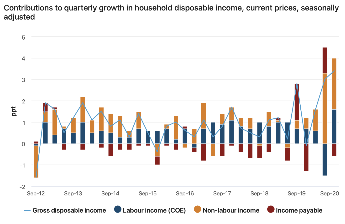
Since there have been few spending options for all that extra income, the household savings rate has boomed. Households have spent $121 billion less than they earned so far this year. We can see just how much the income to households from stimulus spending has exceeded declines in incomes in the chart below. The orange bars are how much non-labour income, which includes government payments, contributed to growth in total household income. In short, disposable incomes are up massively and the main reason is the stimulus cash given to households.
This out-sized stimulus package will have lasting effects throughout the next cycle. We have loaded up households with spending money. We have decreased the interest costs on their mortgages and encouraged them to borrow more money. We have turned off the immigration tap, meaning labour market demands can be more effectively channelled towards wage and salary growth.
To me, it seems obvious that the only thing that can happen is a massive economic surge coupled with rising asset prices. There is even a chance of a "surprise" rise in inflation.
All of this could be seen in advance. Back in May I argued that house prices are more likely to rise than fall, and that most people had under-estimated the scale of the stimulus.
Here's an interview were I explained my reasoning.
The sale price of homes is not the economic price of housing. Prices, in the economic sense, are the relative cost of consuming newly-produced goods and services.
The economic price of housing is therefore the rental price. It represents the price of being housed today. The rental price is what goes into consumption price indexes. It goes into the national accounts to represent housing service production. It is what standard economic theory says is the price of housing.
The sale price of a house represents the purchase of a perpetual stream of housing services. In essence, you are buying the right not to have to rent a home from someone else.
Why is it important that the sale price of a house is not its economic price?
Because sale prices of housing can rise while their economic price falls. The economic price of housing translates into a sale price via other factors.
So how is the sale price of housing determined?
The asset pricing model
The sale price of homes is determined in much the same way that the price of other rights to future income streams; the asset pricing model.
Converting the value of a flow of uncertain future income flows into a capital value today is an imperfect procedure, relying on estimates of risk, uncertainty and growth prospects. But we can for now ignore these judgements to demonstrate how the ingredients that create an asset price from the value of an income stream fit together.
Housing asset prices can be reflected by the following formula.
There are hence five ingredients in asset prices, of which only one is the economic price in the form of the annual rent. This is why housing asset prices can diverge so significantly from rental prices.
Let us go through each ingredient.
Gross rent is the total amount a renter would have to pay to occupy the home for a period. It is the economic price of housing.
Ongoing costs include upkeep of the house—the maintenance required to sustain its current quality over time (depreciation)—as well as other ownership costs such as taxes and fees that are not levied as a fixed rate on the property value.
The risk-adjusted return is the rate of return buyers are will to pay for that property based on their assessment of market alternative investment returns, and the relative rate of risk of buying this house. For example, if you can get a 5% return on you money in the bank from interest, and buying this house is seen as much risker than bank deposits, then this return will be something above 5%, say 8%.
The property tax rate is the rate per dollar on the total property value that is required to be paid in taxes. In most US cities and states, property taxes are levied on the full asset value of the house and land, whereas in other places like Australia, these taxes are levied only on the land value component. I have adopted the US approach here for simplicity.
Growth expectations reflect the rate at which much buyers expect rents or prices to rise in the near future. For example, you may buy a house to avoid paying $20,000 per year rent, but rents might be rising at 5% per year. Next year, your current house purchase saves you $21,000, and it saves you $22,000 the following year.
We are going to simplify this model for now by pretending that growth expectations are zero. This avoids the part of the recipe that leads to big swings in the value of housing that usually self-correct over time. We will also pretend that the risk-adjusted return is best captured by the prevailing mortgage interest rate. Once you see the logic if the model, you can easily tweak these assumptions yourself to see their effect on asset prices.
The cost of buying vs the cost of renting
Here is an example of the asset pricing model in action. A house has the following characteristics.
Rent is $20,000 per year Ongoing costs are $5,000 per year Mortgage rates (risk-adjusted return) are 6% The property tax rate is 0.5% Growth expectations are zero.
The sale price of this home will be roughly $231,000 according to the asset pricing formula [(20,000-5,000)/(0.06+0.005) = $231,000].
What this means is that you will be equally well off economically—i.e. you will spend the same each year—if you borrow the full house price amount and buy it as you would be renting it. We can add up the annual costs of buying to seeing that it is the same as renting.
Interest = $13,850 ($231,000 x 0.06) Ongoing costs = $5,000 Taxes = $1,150 ($231,000 x 0.005) Total = $20,000
You might notice that I have only considered the interest cost of a mortgage, not the total repayment. But paying the principle of the house is not an economic cost. It is an asset investment just like paying listed equities is an investment, not an economic cost.
Our homebuyer in this situation is paying a $20,000 economic cost of housing. But if they pay the principle of their loan over 30 years, the mortgage repayment is $16,780 per year, or $2,930 more than the interest alone. Their out-of-pocket expenses are $22,930, but that include the purchase of $2,930 of housing equity each year.
The effect of low interest rates
Most of the change in housing sale prices over the past decade are not due to the economic price of housing as the chart below shows. Rents have been flat in Australia, and in many cities globally, while sale prices have grown enormously.
If recent sale price changes are not due to rents, then they must be due to one of the other ingredients in the asset pricing model.
We can eliminate the ongoing costs of upkeep. Construction costs have been steady, and fixed fees and charges also have seen little variation. Property tax rates are also relatively unchanged, at least in Australia. Note also that higher property taxes reduce asset prices.
We are now down to two factors—the risk-adjusted return and growth expectations.
It could be that buyers of housing have increased their expectations of rental growth. Though after a decade of flat or falling rents, rental growth expectations should certainly have been curtailed, rather than increased.
This leaves only the interest rate. To me, this is the big story for housing prices over the past two decades globally.
We can take our previous example dwelling where we calculated its value to be $231,000 when mortgage interest rates were 6%. Now, mortgage interest rates are closer to 2%. At what price does buying cost the same as renting at this much lower rate?
Again assuming zero growth expectations, our asset pricing formula is (20,000 - 5,000) / (0.02 + 0.005) = $600,000. That’s a 160% increase in sale price, while the economic price of house remains unchanged.
We can check this calculation to ensure that the economic cost of buying at this price remains the same as before.
Interest = $12,000 ($600,000 x 0.02) Ongoing costs = $5,000 Taxes = $3,000 ($600,000 x 0.005) Total = $20,000
Notice that the interest paid on a mortgage is actually lower in this case, though the annual taxes are higher due to the higher sale price.
What about property taxes?
At lower interest rates the effect of property taxes on asset prices increases. Let us compare the sale price of our example house in two different jurisdictions—one with a property tax rate of 0.5%, and one with a property tax rate of 2%.
First, we can see the effect of property taxes in our high 6% interest rate scenario. Recall that the asset price with a 0.5% property tax rate was $231,000. If we now put a 2% property tax rate in our asset pricing equation, the house is worth $187,500. Compared to this high-tax region, the asset price of the same house in a low-tax region will be 23% higher. That is a huge difference. Yet the economic price of housing is the same.
In the low interest rate scenario our house was worth $600,000 in the 0.5% low property tax area. If we plug in a 2% property tax rate and a 2% interest rate we get a value of $375,000 in the high-tax region. The sale price is now 60% higher in the low tax area for the same economic price of housing. The low interest rate environment amplifies the price effect of different property tax rates.
We can see the components of the economic price in the high property tax area in the low interest rate scenario below.
Interest = $7,500 ($375,000 x 0.02)
Ongoing costs = $5,000 Taxes = $7,500($375,000 x 0.02) Total = $20,000
We can therefore use the asset pricing model to predict that the recently-announced reductions in property tax rates in Harris County (Houston) will fuel price growth in the current low interest rate environment. We can also predict that states like Texas, with comparably high property tax rates (often 2% and above) will have even greater housing asset price divergence compared to regions with low (sub 1%) property tax rates.
Predicting strange price differences
Strange house price differences make more sense through the lens of asset pricing.
Here is an example of the types of strange price differences commonly noted. Hereare two houses where the asset price seems unrelated to the quality or size of the dwelling.
House 1
House 2
Can asset pricing make sense of the fact that the much smaller home is worth nearly double the much larger one?
It can.
We can even acknowledge that the economic price of the larger home is much higher, despite location difference. But this does not have to translate into a higher asset price.
The large home, House 1, might have the following characteristics.
Gross rental per year: $40,000 Property tax rate: 3% Ongoing/upkeep per year: $10,000
The high upkeep costs (aka depreciation) come from its size and features, such as the pool. Notice that property taxes are around $15,000 per year for this dwelling, which is over 3%.
The smaller home might have the following characteristics.
Gross rental per year: $30,000 Property tax rate: 0.8% Ongoing/upkeep per year: $5,000
Notice the much lower property taxes and upkeep costs. This has a big effect when converting the economic price into an asset price.
I’m going to apply a 2% mortgage interest rate to the asset pricing formula to show what price to expect for these two homes.
Although the economic price, the rent, is 33% higher for House 1, this doesn’t translate to asset prices. In fact, House 2 is worth nearly 50% more than House 1 under these conditions (my price estimate is a bit on the high side for both as I’m using a round 2% and ignoring any difference in other asset pricing factors).
Remember, at these prices, each house has the same economic price for buying as it does for renting. House 1 also has an economic price 33% higher than House 2.
House 1 Interest = $12,000 ($600,000 x 0.02) Ongoing costs = $10,000 Taxes = $18,000($600,000 x 0.03) Total = $40,000
House 2 Interest = $17,900 ($893,000 x 0.02) Ongoing costs = $5,000 Taxes = $7,100($893,000 x 0.008) Total = $30,000
If you are not looking at housing sale prices through an asset pricing lens, these strange house price differences will only seem to get worse as we enter a super-low interest rate period. Many people will mistakenly attribute the difference in asset price to physical and regulatory factors, like zoning. But if these factors do affect housing, the must do it through their effect on the economic price, the rent, not the asset price. ____________________________ Next post: Why is the share of income spent on housing so stable over time in almost every place?
Modern housing economists, following in the footsteps of Ed Glaeser, seem to think that the market price of land should be zero. Land only has a positive value because of artificial scarcity generated by zoning laws.
I am not making this up. This is exactly the theory Glaeser has been pushing for two decades.
According to this view, housing is expensive because of artificial limits on construction created by the regulation of new housing. It argues that there is plenty of land in high-cost areas, and in principle new construction might be able to push the cost of houses down to physical construction costs. … this hypothesis implies that land prices are high, not due to some intrinsic scarcity, but because of man-made regulations.
If the price of housing is only the construction cost, that means that the price of the land (location) for housing is zero. It seems a little crazy when you say it this way. Which is why it is usually said in a more sensible sounding “internal logic of my economic model” kind of way. If the input costs to land are zero, and markets are competitive, then the price will converge to input costs. Add in some hedging words, and you begin to sound profound.
But although the model is internally consistent, it is clearly the wrong model. Why?
Land is not a newly-produced good or service, which is the domain of typical economic models of markets, where prices converge to a point that “clears” markets.
Land is instead a perpetual property right to a long-lived scarce asset that can generate income flows. Just like an ownership share of a company, land represents a share of ownership of the finite three-dimensional space.
No one would argue that because there are no input costs for Apple or BHP shares—creating new shares is a legal manoeuvre with essentially no input costs—that competitive trading of these shares will eventually lead to a zero price.
Yet the same argument is thought to be valid when the asset class is land. Maybe if we had public exchanges for land ownership, people would see the commonalities more than they do.
But why can’t land markets be competitive and converge to a zero price? The reason is that the land titles system creates a monopoly over space.
What is puzzling to me is that this monopoly feature of land markets was widely understood issue in the 19th century. It triggered the invention of the Monopoly board game (originally called the Landlord's Game) which demonstrated the monopoly problems inherent to the land titles system and their distributional effect.
Even now, the issue is clear to many who study it. Here’s an entertaining take on the land titles system, and here’s an academic exposé on the issue.
But it remains hidden in the housing supply debate. It is the dog that does not bark in the mystery of rising home prices.
I want to try a new way to communicate the monopoly characteristic of land. The table below shows two ways in which space can be allocated by property titles—either not carved up, with one lot containing all the dwellings on a region, or carved up so that each dwelling sits on its own lot, representing a share of the space. Call it a lot share.
The table also shows two ways in which a property title (a lot or lot share) can be owned—either by a single person or by many people.
If we have one giant lot that contains all the dwellings in a region, and that lot is owned by a single person, then that clearly makes the land market a monopoly. This is a situation similar to company towns, where a company builds housing on land near a natural resource or mine to provide local accommodation for its workers.
Even if that single large lot was owned by many people, such as through a corporate structure, a co-op, or another legal mechanism, it would still be seen as a monopoly.
Although many people own a share of the total space, the space is only one land lot, one property title, so the number of owners does not matter. All the owners’ interests are the same. The monopoly outcome is expected. Even if there are 100 dwellings, with each occupant owning a one-one-hundredth share in the company, it is still a monopoly.
Now let’s carve up ownership a different way. Rather than owning a one-one-hundredth share of a company that owns the single lot containing all one-hundred dwellings, each household ones a one-one-hundredth share of the lot. Rather than subdivide the company structure, the lot structure is subdivided into lot shares.
Each household still owns a one-one-hundredth share of the space.
Does this change to the legal structure of ownership change the economic outcome? If so, why?
In Ed Glaeser’s model world, switching the ownership structure of this area so that each household went from part-owner of the entity that owns the space to part-owner of the space would immediately crash the price of land to zero.
This is internally consistent with his model—land has a positive value only because of “artificial” monopoly features of the market. Once you “create competition” between landowners, prices fall to input costs, which are zero.
One detail that many people overlook when they make the “many owners = competition” assumption is that it is simple for even large numbers of people to converge to the monopoly outcome. Trial and error gets you there. In fact, it is not clear that there is a mechanism that gets a market like land away from the monopoly price. Who would deviate?
This is why, for thousands of years, property titles systems have been stores of wealth—an asset traded in markets and subject to cycles like any other asset class. Thinking about land as an asset explains housing price patterns observed much more than any plausible supply-side story. But unfortunately, admitting that the land market is a monopoly is problematic for economists as it undermines many theories (especially involving anti-trust). It also demonstrates that much of our macro-economic policy—monetary policy, taxation policy, and banking policy— is having large effects on housing markets.
What chance does a political party promising to radically reduce home prices to improve affordability have of getting elected?
The electoral calculus is simple. There’s no chance. If they say they want to, they are lying. This reality is why the Federal Budget included policies to boost housing demand but do not expand the supply low-cost housing alternatives.
The reality is that the richest seven out of ten households own $7 trillion of housing wealth in Australia. That’s $7,000,000,000,000, or seven million-million dollars. Every single 1% price decline wipes off $70 billion from the balance sheets of these households.
Yet we find ourselves in the bizarre situation where politicians are obliged to talk like they want home prices to be lower and “more affordable” but must act in ways that support higher home prices. We can only conclude that our housing market is exactly where we Aussies want it.
Consider these figures from a recent working paper I produced with Josh Ryan-Collins. Bank lending for housing grew from 20% of GDP in 1990 to 80% of GDP today. Business lending for investment grew from 35% to 40%. We have used the power of banking to bid up house prices by trading them with each other while neglecting investment across the business community. No one saw a problem with this because it helped house prices grow.
While the media celebrated the ‘booming’ real estate market, during the 2010s homeownership rates fell from 70% to 65% – back to levels last seen in the 1950s. The main difference between now and then is that governments of the 1950s intervened strongly to get more people into homeownership with public loans for new homes, direct public land provision, and rent controls on landlords that prompted many to sell to owner-occupiers. The state also provided extensive public housing alternatives, with nearly 15% of new supply being public housing in the 1950s compared to just 2% across the past decade.
You can see why our housing situation is so attractive for the homeowning cohort by comparing the economic returns from housing to wages. In the seven years to June 2019, the median Sydney home earned as much from rent and capital gain as the median Sydney full-time worker! This is astonishing. Capital growth of all land, not just residential, went from 9% of GDP on average between 1960 and 1980, to 17% of GDP since 2000, roughly twice the relative return to landowners than just 40 years ago.
Reversing these trends will benefit younger generations who are resigning themselves to the fact that homeownership is beyond their reach. While the “bank of Mum and Dad” has helped shift some housing wealth down the generations, it has entrenched inequalities. Waiting for inheritances won’t work either. The average age of receiving an inheritance is 64 years.
Housing is a defining social issue of our time. We have many technical solutions in our working paper, but the sheer economic value at stake and the political realities of this mean that change won’t be easy.
The problem with making home ownership more affordable is not a small elite locking the majority out: a lot of us (ie homeowners) have a lot to lose if we want to share the joy of a home of one’s own.
Interest rates are the main story for home prices in Australia. With our deregulated banking system, all demand for mortgages can be satisfied (conditional on servicing criteria). With an active and tax-advantaged investor market, this only adds to the tendency for the housing market to converge to the asset-pricing equilibrium, where mortgage interest on the home price substitutes equally for rent, along with some adjustment for ownership costs and expected capital gains.
Here’s the basic gist of the interest rate effect for a typical home that saw rising nominal rents until recently, but where rents are expected to see no nominal growth over the next decade.
Despite rents in this example rising only 47% in nominal terms over four decades, the equilibrium asset price (where mortgage interest substitutes for rent) increased by 338%.
Notice that the 2% point decline in interest rates has a larger effect when interest rates are lower. Halving interest rates should double prices, all else equal (and vice-versa). But that requires only a 2.5% point drop from 5%, but a 4.5% drop from 9%.
The latest bout of monetary policy that took mortgage interest rates from around 4.5% to 2.5% is nearly a halving, which implies scope for a near doubling of prices. Even if Sydney and Melbourne prices were far above the equilibrium due to a recent speculative period, this interest rate decline will bail out speculators and support those higher prices.
This is why I see mostly upside for home prices in Brisbane, Adelaide, and even Perth in the next few years. Gross yields for Sydney and Melbourne houses are around 2.6%. But they are 3.8% in Brisbane, 4.2% in Adelaide, and 3.8% in Perth. A 0.5% point decline in yields in Brisbane, would, for example, see a 15% price gain.
If you can borrow at 2.5% the maths looks like this for a home currently rented for about $400/wk ($20,000/yr).
Annual rent - $20,000 Price at 3.8% gross yield - $526,000 Interest on price (2.5%) - $13,150 Interest on price (2%) - $10,500
If you buy with a 2.5% mortgage instead of renting, you get nearly $7,000 year in your pocket to cover ownership costs and repay the mortgage. If you can get a mortgage interest rate closer to 2%, that gives you nearly $10,000 per year to cover these costs.
Even if you expect rents to fall 10%, this doesn't change the asset-pricing arithmetic much at all.
If you don’t expect prices to fall rapidly, buying makes good financial sense with low interest rates and high housing yields.
UPDATE: It is now cheaper to pay the interest on a mortgage than pay the rent in the major capitals on average (see blue line dipping below one). The below image is that ratio of the interest rate to the gross yield. It also shows the repayment for a 30-year mortgage as a ratio of the rent in orange.
At the current 9.5% compulsory contribution rate, Australia’s superannuation system is already an unbelievably expensive retirement income system. It employs 55,000 people and costs $34 billion in fees each year to deliver only $40 billion in retirement incomes (see the Scrap Superannuation report here). Increasing the compulsory super contributions rate to 12% of wages will do little to support retirement incomes while adding substantially to the economic cost of the superannuation system.
“The economic cost of super to members comes in the form of direct fees, which are around 1% of super balances on average, as well as the foregone investment returns from those fees,” says Dr Cameron Murray, economist and research fellow at The University of Sydney.
“For a typical earner with a 40-year work-life they can expect to have a real super balance of $743,000 at retirement, having paid about $108,000 in fees over their lifetime,” said Dr Murray [1].
“But those fees could have earnt an additional $74,000 in investment income, meaning the total economic loss is $182,000 over a lifetime.”
“Raising the compulsory super contribution rate to 12% will see funds charge this typical earner an extra $28,000 in fees over their lifetime, losing an addition $20,000 of investment income” concluded Dr Murray.
“Even if funds improve their performance and fees fall by half, the compulsory rate increase will see this typical worker lose an extra $16,000 to fees over their working life, and around $10,000 of investment income.”
“The super system is one of the most economically inefficient ways to support retirement incomes. Raising compulsory contributions will only add to these costs, creating even more jobs for blow-hard spreadsheet monkeys who pay themselves from our retirement savings.”
______________________________
[1] First ten years of work-life at 70% of average full-time wage, and last ten years at 30% above the average full-time wage, with middle twenty years at the $90,000 average full-time wage. All returns and costs are in real terms. See Table 1 and 2 for a result summary.
You are a housing developer with a large plot of land on the fringes of a major city with no planning constraints. How quickly should you sell these lots to supply them to the housing market?
This is the question I answer in a new working paper entitled A Housing Absorption Rate Equation (now published here). I sketched out some of my initial thinking on this topic in a blog post earlier this year. Here I want to explain this new approach more clearly and show why it is important for the housing debate.
Why is this important?
Economic analysis of housing supply is usually based on a one-shot static density model. In this model, landowners choose a housing density that maximises the value of their site. The density that achieves this is where the marginal development cost of extra density equals the marginal dwelling price. Every landowner does this instantly. There is no time in the model. It just happens.
But optimal density (dwellings per unit of land) is not optimal supply (new dwellings per period of time).
Despite this conceptual confusion, radical town planning policy changes have been proposed around the world. By allowing higher-density housing, proponents of these policies expect that the rate of new housing supply will increase enormously, reducing housing prices.
I wouldn’t be that confident. It is not clear that the economic factors that influence the optimal density are the same ones that affect the rate of new supply, or what is known as the absorption rate.
What factors influence the optimal rate of supply?
To answer this, we break apart the time dimension of the development problem. In a dynamic setting, the economic value from a sequence of dwelling lot sales is maximised when delaying the marginal sale into the next period makes you equally as well off as selling that dwelling today.
The economic factors that influence the absorption rate are those that change the relative gains from selling now rather than delaying and selling later. Let us think about the motivating puzzle of a housing developer selling new lots.
From the perspective of the second period, if you sell a lot today, you get the interest rate on the lot value, plus you avoid any taxes on that lot value.
If you sell on that later period, you got the value gain of the lot. This value gain comes from the market at large (i.e. the trade of existing dwellings) but is also affected by your own sales in the first period. Sell more now, get lower price growth and hence a lower price in the next period. The net price gain is, therefore, market demand growth minus your own-price effect on that price growth.
The optimal point is where you are equally well off making the same number of sales in the current period and the next period.
The result of the dynamic supply problem is this equation.
Let's walk through this one parameter at a time.
Price growth sensitivity to own-supply, a
The first parameter of interest is the own-price effect, a. A higher a means that each sale today has a larger effect on price growth. It’s a measure of the “thinness” of the demand side of the market. Since a is the denominator, it means that the thinner the market, the lower the optimal rate of sales.
Market demand growth rate, d
When demand growth is high, you sell more. This makes sense. You sell into a boom and withhold sales during a bust. This is important because one argument for relaxing density restrictions is that new supply would occur at such a rapid rate that prices would fall. But falling prices reduce supply. There is hence a built-in ratchet effect in housing supply dynamics.
Interest and land tax rates, i and 𝜏
These two rates work in combination. The interest rate is the gain you get on the cash from selling a lot today, and the land tax rate is a cost you avoid from selling today. The gain from not owning land (i.e. selling it) is the interest rate and the land tax rate, which is positively related to the optimal absorption rate.
The efficiency of higher density, ω
The final piece of the puzzle is the ω parameter. This parameter captures the idea that if you delay selling a lot you can change the density of development in response to rising prices. Remember that static density model? This is where it is useful. It shows that if prices rise, undeveloped sites rise in value more than the dwelling price because the higher price justifies denser housing development.
I show this in the below diagram. At price Pt the optimal density is Dt, and the site value is the orange shaded area (the dwelling price minus the average development cost times the number of dwellings).
If prices rise to Pt+1, then the optimal density is now Dt+1. The value gain for the site is not just the area marked A, which it would be if density was fixed. It is the area A plus the area B, minus the area C. Since B > C this means the site value rises more than the dwelling price change. The ω term captures how much bigger A + B - C is than A. When ω is 1, it means that density is constrained to Dt and site value rises only by the dwelling price change. Flatter cost curves create a larger ω.
The important thing to remember is that constraining density makes ω smaller (holds it at 1). This increases the optimal absorption rate because it reduces the gain to delay that comes in the form of the ability to vary housing density.
Where does this model leave us?
Having a simple absorption rate model allows housing researchers to think more clearly about the economic incentives at play for housing suppliers. It allows us to break away from the “density = supply” confusion. Instead, it focusses attention on the key issue of the relative returns to delaying housing development.
Any policy that increases the cost to landowners from delaying housing development will increase the rate of new housing supply. For example, higher land taxes and interest rates.
Another way to increase the cost (reduce the benefit) of delay is restricting density. This goes against the intuition of most housing researchers, but the economic effect is real.
Think about it this way. You announce a policy that will limit density in an area to half of what is currently allowed in five years time. What happens? You get a housing development boom as projects are brought forward in time. You massively increased the cost of delay.
It is obvious that planning controls change the shape of cities. They reduce housing density in some areas and restrict certain uses in others. That’s what planning does. But how this translates into an effect on the rate of new housing supply across a city is far more difficult to ascertain. This model goes some way to helping housing researchers clarify their thinking about the economic incentives at play in housing supply, instead of relying on intuition and inappropriate static models.
Recent Twitter exchanges have helped me to understand a couple of additional confusions in the housing supply debates. Let me take them one at a time.
The housing supply mechanism
I dunno, man. There's a golf course just down the road from me where I live in SE London. That land would be worth 10-20x as much with permission-to-build. You can argue that a massive increase in building wouldn't affect *prices* much but arguing nothing would happen is crazy
— no employers, don't google me (@sudonimbus) August 17, 2020
This Twitter statement contains some hidden assumptions and two main points; 1) that land is worth different market value depending on the rights attached to it, and 2) that massive amounts homebuilding will affect prices.
Points 1) and 2) are correct. But the hidden assumption that because land has a different value with a planning permit (or with different zoning) that overall homebuilding rates will rise if a plot is rezoned. This part of the mechanism is wrong, in my opinion.
It is not obvious to me that changing planning will greatly affect the rate of market supply. If you assume that planning is the reason new housing supply is not higher, then you are assuming the outcome. I don’t think it would do much at all.
This challenge was put to me.
Let's hypothetically suppose that a new regime grants permission to build literally anything up to 10 stories and compliant with building control on any site within 30 miles of Big Ben.
What happens, in your model?
— no employers, don't google me (@sudonimbus) August 17, 2020
I responded that not much would change.
Let us be clear. Many cities effectively have this type of planning system. Sydney councils, for example, allow tall towers in vast areas of the city and had record new housing construction for nearly a decade. That doesn’t stop people from saying these new apartments should be taller, or that supply isn’t a problem.
Sure a large scale planning change would be a shock to an equilibrium. It will probably stimulate a flurry of activity—site trades, new types of development proposed, and maybe extra buying of these new dwelling types. During this adjustment period, prices would probably rise rather than fall, as is usually the case. But this would quickly calm down until there is no sustained change to the rate of supply.
The effect will be like any other small shock to a dynamic system.
Developers slow their sales when prices fall, and increase them when prices rise. They build to order. I do not see what mechanism there it so sustain faster supply and falling prices with these economic dynamics at play. Would it make sense for any developer to sell out their apartments at lower and lower prices to sustain a faster sales rate?
The zoning and land value issue
Additionally, the fact that changing zoning, or permitting development, affects the price of a property seems to be evidence about supply constraints for many people.
Not sure the blog helps the author’s argument, as 1) land values and changes in value differ hugely depending on housing permission rights, that supports @s8mb point about interest rates 2) density of rental accom (people per flat and location rel to Work) have deteriorated
This exact argument was the second paragraph of a recent RBA paper about housing supply.
There is a hidden assumption at play to make the leap from “different property rights have different values” to a supply shortage. Unless you want to argue that property rights should have no value, then this is a weird argument.
No one would think it unreasonable that if you gave a landowner the rights to use adjacent public space to build extra housing that their property rights would have a higher value. Yet when we change the orientation of neighbouring rights from “beside” to “above” apparently these rights should be worth zero.
We know rights to airspace and higher density are valuable because they can be traded in some markets. They are a distinct property right. Planning is a tool to allocate them.
There are no "true" property rights to land that go from earth to the heavens. With property rights, you get what you are given.
Strangely Ed Glaeser’s approach to housing implies that property rights to land should be worth zero. He says, in essence, housing supply would be effectively unconstrained without planning and land values would fall to zero.
He is careful not to say it this way because it sounds stupid. He instead says that the cost of housing will be pushed down to construction cost. Hence, the land component of home prices will be zero.
This is unusual, to say the least. It implies that if you removed all planning controls (build anything anywhere) that land would become valueless. If this were true, announcing such as policy would crush land value to zero immediately as expectations get factored in. Who would want to own an asset whose value is rapidly trending towards zero?
How you can affect housing prices with “supply”
On the Jolly Swagman podcast I thought I understood you to be saying that housing supply is not the main issue. But then you also mentioned flooding the market with new stock would help and also that artificial drip feeding impacted prices?
The physical number of homes does not change prices much. It was, therefore, confusing to some when I said we could flood the market with supply to reduce prices. If we think about property price crashes, we can see what flooding the supply-side of the housing asset trading market can do. This effect has nothing to do with the total quantity of dwellings. In fact, such price declines are usually accompanied by crashing housing construction.
I also do not claim that developers artificially drip-feed new supply. There is nothing artificial about it. This is the normal market outcome. Another way of saying it is that there is a rate at which they must sell to maximise the value from their land. If the sold faster, they would undermine their own profitability, which would happen because these faster sales had an effect on price. When I looked at developer landbanks and sales data it was common for large approved (<200 lot) subdivisions to go a full year without a single sale. If they wanted to sell, say, 10 lots that year instead of zero, they would have had to drop the price substantially.
"Flooding the market" can be thought of as mimicking the asset-trading dynamics that happen during a house price crash by adding many desperate sellers to the market. A public housing supplier could do this. The scale would have to be very large, but this is exactly the large scale change in supply many expect to happen automatically from rezoning. So why not guarantee that it happens with a public competitor to these private housing suppliers?
An improvement on this "flood the market" idea is to copy how the price of money, the interest rate, is regulated by central banks. They promise to supply reserves (and demand back reserves) at narrow price range around their target rate. Their promise to back these guard-rail prices with a supply of reserves is enough for private market participants to adopt that price. In effect, monetary policy is implemented by announcement. They rarely have to use the guard-rails because they are credible.
Imagine a Central Housing Bank (CHB) with a promise to buy any dwelling at a $300,000 price and sell as many dwellings as desired at $310,000. Obviously, it would be more sophisticated than this with price schedules for different locations and dwelling types. But regardless, it sets a price corridor with a price promise backed up with an ability to supply housing.
If this institution demonstrated its ability to back up its sales with new housing, this credibility would lead the market to accept that price and operate within the corridor. It would realign market expectations on prices and capital gains.
How many new dwellings would need to be built to back up that promise and demonstrate its credibility? Probably not as many as you would think. Yes, there would be waiting lists at first as home production ramped up to back up those sales. But even then there would still be an effect. Pay $500,000 or wait a while on the waiting list and pay $310,000?
I would guess that building about 30,000 thousand dwellings per year for the first few years in Australia would make the CHB credible. Maybe 60,000 per year in the UK.
Now, I do not think this is the best “solution” to high housing prices. I think the best affordable housing system is Singapore's proven model.
What thinking about this option does is show that we do intervene in important asset markets, like money, when we think a different price would be socially more desirable. It also shows how difficult it would be to get prices down via supply-side interventions.
It also puzzles me that those who want low home prices and think homebuilding will get us there usually do not advocate for such systems. Why not advocate to copy Singapore’s model to build every citizen a new home at construction cost? Why not propose to flood the market via a non-market housing developer who will meet their supply targets regardless of how low they have to drop prices?
This report, entitled Help to Build, is apparently a plan to support housing supply, yet it proposes only demand-side interventions. In effect, it concedes that housing supply responds to demand and that we just need more demand to get the supply. If this is true, then it cannot be true that planning changes will result in voluntarily faster supply at the same level of demand.
Likewise, suppliers are unwilling to ramp up output unless they think there will be a prolonged period of high demand since they do not want to start up only to have to switch off shortly after.
This is a long post, so I will stop. Post your questions in the comments.
Sam is right about some things but wrong on most. So let’s try and pin down our disagreements.
Let me first disclose my professional background. I have worked for listed and private residential and industrial developers and worked for the state regulator on infrastructure charging regimes. My first degree was in what was a then niche area of property economics, covering a range of topics involving construction management, design, town planning, feasibility methods. My PhD included extensive analysis of planning decisions, and I have published many academic papers on housing, planning, and supply dynamics. I have also been an expert witness in corruption cases involving town planning decisions.
I can assure you that if there were an issue with the planning system constraining the rate of new housing supply, at least in Australia, then I would be spending my days arguing that case.
Let me also say that I am not anti-supply. I do think the planning system is more cumbersome and costly than it needs to be, even in most jurisdictions in Australia. But I don’t think that changing the planning system is going to do anything about the overall price level of housing. I support public housing supply programs that have clear objectives and penalties for missing targets.
I like to preface any housing supply discussion with a thought experiment to help disentangle whether housing issues are mainly about distribution or supply. If every mortgage was written off, and every renter was given the home they currently live in for free, so that 100% of households lived rent- and mortgage-free in their current homes, would there be a housing affordability crisis?
I’ll leave that with you.
Sam makes nine arguments against certain claims of "shortage deniers". Please go and read them in full.
“House prices are high because of interest rates, not a lack of supply.”
“Rents haven’t been rising as a share of income, so there is no shortage.”
“The elasticity of house prices to new supply is low, so building more houses won’t do much to lower prices.”
“Nine out of ten planning applications are granted, so the problem isn’t the planning system.”
“Land banking is the cause of housing shortages.”
“Empty properties make the housing shortage worse.”
“The private sector cannot build enough houses to meet demand.”
“It is impossible to make housing “affordable” without council housing / affordable housing.”
“We risk speculative development after building booms which leaves us with ghost towns.”
These are my responses.
Low interest rates
On this issue, I think we mostly agree. Low interest rates increase the price of assets by reducing the capitalisation rate.
We differ on this part of Sam’s explanation.
"Falling interest rates do not increase the price of other durable goods like airplanes or ships, or of housing in places where there is not a supply constraint, like in the North of England or Houston (which has a liberalised planning system)."
The missing distinction here is that housing is a durable good attached to a property right to a piece of the three-dimensional space that has been carved up with a land titles system. Home construction has not inflated in price, just like other durable goods. But the cost of buying a share of the property rights system from the system’s existing owners has inflated. Without that, you have nowhere to put your dwelling.
We can, therefore, agree that the problem has something to do with property rights having perverse effects. Sam thinks it is the permitting part of the property rights system. I think it is the property titles system itself.
We also disagree on this point.
“If interest rates were the only factor, we would expect to see houses everywhere rise and fall in line with them.”
No. We would expect to see the interest rate effect on the capitalisation of rents the same everywhere, but with prices still diverging due to non-interest rate factors. Different cities have housing price booms at different times for different reasons. Houston’s 1980s price boom is a classic example of a price boom that far exceeded that scale of price growth in other cities at the time. There were other factors at play, including plain old expectations and speculation.
Sam's own chart seems to show that most variation in prices is common between London and the rest of England.
Rents as a share of income
I think we agree here that rent is the appropriate measure of the economic price of housing, which is good.
Sam’s view here mainly deals with UK rental statistics. I would defer to Ian Mulheirn who has two detailed pieces about that issue (one and two).
But we differ on this point.
“Suppose everything we spent money on changed in the same way, rising in real-terms as we got richer – groceries, electricity, clothes – without getting any better in quality. Economic growth would be meaningless, because any overall income growth we experienced would simply be eaten up by these rising costs.”
Remember my earlier point. Housing products have not increased in value in line with incomes. The combined cost of renting houses and that location in the property titles system has grown in line with incomes. Remember also that this location rental is also someone’s income.
What makes property different? When you rent a dwelling you also rent the location, essentially buying out your transport costs by paying the owner of a better location. If we had an equilibrium where people spent 5% of their income on rent, some people might start deciding to spend 7% of income on rent (40% more rent) to live in better locations rather than spending that money and time on commuting. Those with higher incomes will find that the time-cost of commuting is relatively higher, with the equilibrium process sorting the location of households by income or wealth at their maximum willingness to pay (taking into account the cost of transport).
Compared with tradable and transportable consumer goods, it is the finite nature of locations and their relative advantages that ensure we end up in a fixed-share-of-income equilibrium.
The way to use rent-to-income as a supply metric is to see whether the number of people per dwelling is increasing compared to the average size of dwellings. A shortage would be indicated by more people in smaller dwellings paying the same share of income on rent.
It may be the case that this exists in some locations but not others. The question would then arise, how does this situation persist if there are alternatives in different locations — just pay the lower rent plus higher transport costs and get more space.
These are the types of questions and the evidence we should be looking about when talking about the adequacy of housing supply.
Elasticity
It is also good that we agree that the price elasticity of housing supply is low.
Sam says the following
“Imagine a similar argument being made during a famine where the price of food was very high: if an additional food shipment did not make a big dent in overall prices, would we conclude that the solution wasn’t more food?”
Yes. That’s right. This evidence would force you to conclude that although more food would be beneficial, the distribution of food is mainly causing the famine because adding more total food to the system is not helping much. This very point is the subject of many debates about famines and food prices. It is also why I prefaced this piece with a thought experiment about the distribution of dwellings.
Regardless, saying that more dwellings won’t decrease prices is wrong. What Ian Mulheirn and I are saying is that because housing supply matched population growth, and in many places far exceeded it, that supply is not the cause of the price growth observed. Adding more supply will decrease prices, (putting aside whether changing planning rules actually will change the rate of supply). But it happens in a slow and expensive way.
In Australia, around 8% of the labour force and 6% of GDP is spent on building new homes. When someone says “let’s double housing construction” from 1-2% of the stock per year to 2-4% of the stock, they are really saying “let’s take 8% of the workforce away from what they are doing to build more housing for a 1% rental price decline each year”. Maybe that trade-off is worth it (assuming supply would increase this much by removing planning regulations). Maybe not. But this is where you should end up when talking about elasticity and the size of the price effect of the investment in new housing.
High approvals rates
I agree that this metric cannot show the effect of deterred planning applications.
But does that make it meaningless? I don’t think so.
In a radical supply shortage situation, with so much profit to be made from getting into the housing game, even low probability applications would be made. People buy lottery tickets all the time. Large organisations often invest billions in activities with low probability outcomes when there is a large potential payoff.
Shouldn’t we see the planning system swamped with low probability applications and observe them being rejected?
I also have a gripe about planning applications and their apparent slowness. While the situation is different in the UK and Australia, slow approvals usually happen because the applicant has sought approval for a development that is far outside the scope of the plan. They bought land that was not designated for what they wanted to build, then chose a slower route through the planning system rather than a faster one. I'm surprised that these developers have the confidence to blame someone else for their self-inflicted problems!
Land banking
Sam writes that land banks are an inventory necessary to smooth out supply and ensure workers are not idle after selling stock.
I agree that land banking smooths out supply.
I disagree that land banks are inventories. I even have an academic paper on this topic where I looked at the annual reports of listed housing developers to see what they say to investors about planning when they are obliged to be honest (here's a free working paper version). Australian developers never seem to tell investors that planning is delaying them.
We are now getting to a key issue on housing supply. How does a developer choose the rate per period to sell their subdivision?
They need to be careful not to sell too fast. Faster sales might require lower prices, or raising them more slowly, reducing the present value of the return from that project. But if they wait too long, they might also miss out. As I often say, what kind of crazy property developer floods the market because they can?
I also don’t see how land banking is a symptom of a shortage. In any other product market, even large durable goods like ships or trains, large inventories don’t happen when there is a shortage. Do these firms “buffer” and keep large inventories to smooth out their production? Most large capital goods production is on a “build to order” model where the process schedules buyer orders, matching supply to demand.
Empty properties
I have no idea how many empty homes there are in London. Sam seems to have the data. I can attest to the fact that Australia has more empty homes as a proportion of total dwellings now than at any point in history, along with larger homes and fewer people in each one.
The private sector cannot build enough / need council housing
I agree with Sam that the private sector can build enough homes. I disagree that they would just because they could.
I love how all the housing supply people bang on about planning, but almost never propose that the government should build so many houses that prices collapse.
You know, just in case private developers choose not to collapse the housing market by flooding it with new supply.
I am quite often puzzled that using the power of government to flood the market with housing is never proposed. We just cross our fingers and hope that the private sector will crush the price of their assets.
Sam has stumbled across the “absorption rate question”. How fast should developers build to maximise the present value of the flow of their economic returns from development?
Clearly, it is not so fast that the final sales of a subdivision are at a far lower price than the first sales. This would also see problems with buyers pulling out of contracts and purchasing at the lower later price.
If we look historically, periods of rising homeownership and rapidly expanding supply are usually associated with government programs—housing for returned soldiers, giving public housing to tenants, Singapore's subsidised housing model, and so forth. My view is that we should expand these programs just in case the private market doesn't deliver what it promised. Think of it as insurance.
We risk ghost towns
I don’t think already large cities are going to risk this, so I agree with Sam that this is a silly argument.
I would only note that this happens in places like mining towns where they really do see rapid demand growth—expressed in rents—along with high and unconstrained rates of new home building. Of course, despite the lack of supply constraints, mining towns always seem to still get a boom and bust rent and price cycle. I wonder how Sam would explain this.
A puzzle came via twitter following the crazy story of RBA research claiming that if you remove planning controls, apartment prices will fall 42%.
I argued that it would be weird for property developers to lobby for policies that eroded the value of their products and sent their housing projects broke.
Andrew responded as follows:
Equally, do you think that NIMBYS aren't arguing for restrictions that increase the value of their land?
It seems pretty obvious to them that if they restrict higher density in their area and force it on other areas the value of their land will increase.
So we have two groups who apparently stand to benefit from tight planning controls if they do in fact increase prices, yet they are arguing opposite cases.
This is a genuine problem. How do I make sense of it?
The first thing I would do is break it down further. Homeowners are an investor-renter hybrid—landlord and tenant of the same property. Maybe we can break out renters and landlords separately and see if they lobby for different planning outcomes. The position of homeowners would then reflect them acting as their “renter” or “landlord” selves.
Survey research has shown that renters are just as likely to oppose rapid development in their neighbourhood as homeowners, perhaps even more so if we believe this survey.
“If a similar ban were proposed for your neighborhood, how would you vote?”
Given the consistent NIMBYism found among homeowners nationally, I expected homeowners to show stronger support for a ban on new development within their own neighborhood. Instead, only 40 percent of homeowners chose to support this ban compared to 62 percent of renters. In other words, 30 percent more renters supported the NIMBY ban than homeowners.
This gels with my experience in community groups. Renters play a large role. Investors/landlords not at all.
If tight planning controls increase prices, renters will be the worst off, having to pay higher rents. Yet they lobby in favour of these tight controls.
Landlords will be better off, but they do not lobby in favour of tight controls.
So if homeowner NIMBYism matches the behaviour of renters, not landlords, then we can say that NIMBYism is not financially motivated by homeowners looking to increase the value of their homes.
NIMBYism is part of what drives property prices so high. When opposition to local development means that homes can’t be built in useful areas, the remaining homes become scarce and extremely valuable.
So what’s the deal?
One way to reconcile this behaviour is to question whether in fact tight planning controls increase local rents and prices. My experience as a property developer is that areas undergoing rapid densification become more attractive and, if anything, increasing in value.
Some have argued that it is the risk, or variation of the outcomes, from densification that homeowners don’t like, hence their conservative status quo bias. Will the benefit of more local retail services outweigh the cost of extra traffic or not? This risk issue could certainly be part of the story.
Another resolution to the puzzle recognises that densification typically does increase local rents and prices but, unlike investor landlords, homeowners can’t realise any financial gains without selling and relocating.
Since they chose to buy and live in their suburb rather than an alternative area, they have a preference for the current density/amenity. Had they known they were buying into a high-density area that was not yet built, they may have chosen to buy elsewhere instead. The same logic applies to renters.
It would be a bit like someone coming along and offering to paint your car pink. Sure, maybe pink cars sell for more, but if I wanted a pink car, I would have bought one in the first place.
If NIMBY psychology is more like this, we would expect that development that complies with zoning codes to see little push back, as homeowners have reasonable expectations about what sort of development is planned for their area. But we would expect a lot of push back against development proposals that fall far outside planning codes. This is consistent with my experience.
In the end, I don’t think I am fully satisfied with any of these ways to reconcile the NIMBY and developer puzzle.
What is clear is that the story is not a simple one of NIMBYs preventing some local developments in order to increase the value of their home.
What are your thoughts?
fn. [1] The conventional wisdom is often wrong when it comes to property markets and planning.
The NSW government has been conducting a review of taxes and federal financial relations. One of the main proposals to come out of the review has been to replace stamp duty on property transactions with a broad-based land value tax, or what I have called SD4LVT.
There are many reasons to be sceptical of the political motivations of these types of reviews. Typically, you only undertake this type of drawn-out review process if you a) already know what you plan to do, or b) plan to do nothing but use the process to keep all the interested parties busy talking about something that will never happen while appearing to do something.
I think this is a case of a). I say this because although the review proposes SD4LVT, the NSW government recently announced that it will be reducing land taxes by 50% for 20 years for corporate landlords. The reason given is to promote a corporate build-to-rent housing sector [1] which is currently disadvantaged because there are threshold values above which land taxes apply, giving a tax advantage to landlords that own few properties.
But if the NSW government wants to expand land value taxes, why offer additional exemptions and reductions to fix the imbalance rather than remove the current exemptions to level the playing field?
So I'm a sceptic.
Regardless, the SD4LVT proposal has been justified with a lot of dodgy economics. I outline in my submission four main areas where the economic reasoning is flawed.
The economic efficiency costs of stamp duty are low, not high.
Removing stamp duties may increase the price of housing.
Lower churn of housing assets is an economic benefit of stamp duty.
Stamp duty revenue volatility helps stabilise the macroeconomy.
Please read the whole submission. Here's an excerpt about the nonsense economics that is behind the conventional wisdom about the high efficiency costs of stamp duty.
_______________________________
The metrics of economic disaster caused by stamp duties are derived from economic analysis using computational general equilibrium (CGE) models of the macroeconomy. The below table from the Draft Report shows that multiple assessments conclude that there are high economic costs to raising revenue from stamp duty.
However, these studies all use CGE models that assess the effect of transaction taxes because there are no transactions in the models. Instead of using a better tool for the job, or admitting the limits to knowledge, modellers have simply pretended that stamp duties are a different tax that applies to a tax-base that is in their model.
There are two main approaches to this. First, in the KPMG models, rather than stamp duty being a transaction tax that is incident on the seller (and therefore incident on land values), as it is in reality, they assume this instead.
...conveyancing stamp duties are modelled as a tax on investment in residential and commercial structures (p.125)
They assume that stamp duty is not a tax on transaction where the economic incidence is on land. Instead, they assume that stamp duties raise the cost of housing to all buyers and renters because it is a modelled as a tax on construction. The model assumption requires that stamp duties raise the cost of building new houses without affecting land prices, leading to reduced new housing construction in general. This is a classic example of garbage in, garbage out.
A second approach is in the COPS model is to pretend that stamp duty is a tax real estate agent fees and legal services used in housing transactions.
Stamp duty on conveyancing or property transfers in Australia are taxes that apply to the transfer of ownership of most properties. While the duty base is the sale value of the property purchased, the resources used in transferring property ownership is usually only a fraction of the value of the property transferred. To model transfer duties on residential property ownership in this way, we introduce a new bundle of goods into the household decision problem in VURMTAX, called Moving Services. This bundle consists of goods produced by the Real Estate Services, Other Business Services and Public Administration industries, and represent the real estate agent, legal and public administration goods demanded by households when transferring property. (p17)
...we have $8,367 million of stamp duty being levied on an activity with a resource cost of only $1,881 million. This implies a tax rate on the activity of transferring property of 445 per cent (=8367/1881). (p.804)
This means that instead of the tax being a small percentage of a large base (property turnover value) they are instead suggested that the tax is a 445% tax on real estate agents and conveyancing.
If that sounds crazy, that’s because it is. Any tax at this rate is going to look costly and inefficient in a CGE model. The more bizarre part of it is that if you believe this modelling approach is an accurate representation of stamp duties, then the cheaper real estate agents and lawyers become, the more economically inefficient stamp duties are.
The claims about the economic inefficiency of stamp duty that are relied upon to justify its removal have no plausible economic basis.
_____________________________
[1] I've never understood what is supposed to be achieved by this. We currently have a rental market ownership structure of "investor owns dwelling." What is achieved with a structure of "investor owns shares of a company that owns dwellings?" On net its the same. I could be convinced that landlord professionalism could be improved. But again, most landlords employ profession property management services anyway.
Twitter is a mob, and the mob has a new enemy. Professor Gigi Foster has been on a few television shows lately trying to make the case that economic lockdowns cost lives, just as COVID does, and therefore we want to make sure that we aren’t inadvertently killing more people over the long-term by crushing economic activity and livelihoods.
After all, a functioning economic system is what delivers high-quality healthcare, safe roads and workplaces, investment in public works, the ability to devote resources to research medical treatments and new drugs, and more. It delivers livelihoods and careers, leisure and happiness. It delivers quality of life as much as it delivers quantity.
However, I don’t think gotcha television and infotainment current-affairs shows are the best venues for this discussion. From what I saw, these outlets were actively avoiding putting a number on the trade-off, or even acknowledging it. A cabal of social media economists avoided acknowledging this trade-off a few months back. They then back-peddled, said there was a trade-off, and botched their attempts to quantify it.
The puzzle to me is that everyone seems to want to say Gigi is trading off lives for the economy. Her point is that a functioning economy delivers health and welfare outcomes, and hence the trade-off is about lives for lives.
For some reason, saying this is a new taboo.
Policy decisions that explicitly make this trade-off occur all the time. Should we fund more medical research? Should we install traffic lights? Should we make people wear seat belts? Should we ban alcohol and cigarettes? Should we legalise recreational drugs?
Policy analysts, particularly economists, spend careers looking at these welfare and livelihood trade-offs in all sorts of policy domains.
When she says "man up" she means that we need to face up to the fact that we cannot create a pre-COVID world. There are going to be losses of life quality and quantity, either from the virus or our response to it.
I want to go through some of the strange things I see when talking about our COVID policy response, and some of the things people say to avoid facing the reality of this trade-off. My personal view is that the reasonable thing to do is to make sure our policy response does not shorten lives and reduce their quality more than COVID would. I hope that this helps people to understand where Gigi is coming from.
1. The exponential growth and tail risk story
One of the big claims early on was that those talking down the risk didn’t understand exponential growth. Strangely, exponential growth doesn’t usually apply to virus propagation. The pattern is well-understood to be logistic growth, which is going to saturate the population at some point. The unknown was merely where that point would be. An upper bound for that point was pretty clear early on based on evidence from China, Italy and the Diamond Princess cruise ship.
2. Virus prevalence estimates
How much of the population has been exposed to the virus? This is another area where the worst-case scenarios got all the airplay, and where more sensible estimates were ignored. The more prevalent the virus was, the lower the overall mortality. You can see the media incentive for publicising the high mortality estimates, even though it was known quite early on what the realistic estimates were.
3. Infection and case fatality rates
Initially, the highest estimates were promoted, but the reality is that the range of 0.25-0.65% for infection fatality is the current view. If two-thirds of the population is infected overall, that is a worst-case scenario of about 0.16-0.4% of the population dying from COVID, or a few months of normal deaths brought forward in time. This is a generous worst case. The "Swedish disaster" has seen a crude COVID death rate of just 0.05% of the population, under a third of my lowest estimate.
4. Getting the orders of magnitude right
I asked my Mum when she was panicking about the COVID outbreak how many people she thought had died. She said 5.
When people tell me about the shocking number of COVID deaths I like to ask them how many people die each day in normal times. No one seems to know, or care.
Nearly 8,000 people die every day in the US. Fear does not care for statistics.
The 6,000 coronavirus deaths likely to come from the virus in Sweden are equal to around 24 days of normal expected deaths, and many of these COVID deaths are not in excess of normal deaths.
A good rule of thumb is that 8 in 1,000 people die every year (0.8%), or about 60 million globally.
For perspective, the seasonal flu in Australia kills 1,500 to 3,000 people, with about 18,000 hospitalisations.
In Queensland alone last year 285 people ended up in ICU due to flu.
5. Getting the cost of life right
Everyone dies, so dying of one thing today simply stops you dying from something else later. Deaths are life-shortening. In the trade-off I described above, economic recessions and lower future output are also life-shortening. There is no point talking about “prevented deaths”, only shorter lives (that whole quality/quantity thing). If people die a year to two younger than otherwise from COVID, then that’s not too bad. If they die 30 years younger than otherwise, the loss is fifteen times worse per death.
6. But what about transmission!
Another argument is that coronavirus can have lasting effects on some people. Yes. And? Others say that you might feel bad transmitting the disease to others. Yes. And? These issues are true of all viruses. They were true of last year’s record 1,300 flu deaths. There are hundreds of people out there who transmitted the flu virus to someone last year and it killed them. Where was the outrage then?
7. Or do recessions save lives?
I’ve heard the argument that recessions decrease traffic and workplace fatalities, reducing crude death rates. I can’t make a judgement about whether this is true, but it makes perfect sense and could be. But it only raises another question—if recessions save lives as a general matter, why aren’t we trying to orchestrate recessions all the time? If it is logical to do it for coronavirus, then it is logical to do it for traffic fatalities, workplace deaths, or whatever other indirect mechanisms of death are at play during economic expansions.
8. The poorest countries suffer the most
There are global costs to lives from large scale lockdowns. Global vaccination programs for preventable diseases are being delayed, costing lives right now. Construction of health facilities is being delayed, costing lives in the future. Their general development and progress are hampered. Worse still, with very young populations, most poor countries have relatively few people at risk of COVID.
9. The endgame. What endgame?
After a month of “flatten the curve” rhetoric, which basically had the right intention, there was a silent shift towards “crush and eliminate”. How does this make sense in a globalised world where the virus is going to saturate the rest of the world population? What endgame does that entail?
Being a national bubble with no international travel for years until a vaccine adds to the human cost of our policy response. If (or when?) the bubble is breached we get outbreaks anyway. New Zealand is hailed as a success on this front. But until when? The first person who arrives with COVID will simply take NZ back to square one.
10. The counterfactual
This is tricky to consider. Is there a “no panic” counterfactual where the media doesn’t whip up society into a frenzy? I think there is, and this means that the “people would voluntarily lockdown” argument doesn’t fly. Why would they voluntarily lockdown?
The 2017 flu season was nearly 4x worse than the 2016 flu season, with 1,255 deaths compared to 464 the prior year.
In relative terms, the 2017 flu season was huge. It also had the risk of being multiple times bigger given the state of knowledge in the early stages. Yet no one panicked and shut down society.
If people don’t notice a 4x jump in flu deaths, would they notice a 10x jump from coronavirus deaths and voluntarily lock down? I argue they wouldn’t.
The “don’t panic, don’t lock down, invest in health resources” counterfactual is a plausible one.
11. The un-science cancel culture
The Twitter mob has decided it can decide what is science and what is not, while at the same time attributing all variation in the COVID outbreaks across different countries or states to the policy response, leaving no space for randomness or luck.
This is “un-science”.
There is also nothing the un-science mob loves more than cancel culture. If my Twitter searches are anything to go by, plenty of people now want Gigi to be fired from her job. Yes, for raising the point that we should try and save the most lives possible by accounting for the cost to lives from our response to COVID, she is apparently now someone who can justifiably be cancelled.
12. A final thought
One thing I have learned to do to help maintain perspective is to turn a problem around and ask the reverse question. How many early deaths would we tolerate to avoid a large recession? Is your answer really zero? Even a global one?
How many early deaths do we tolerate by not spending more on the public health system? Where is the outcry?
[UPDATE]: After being hailed as a success story, on August 13 New Zealand went into a second lockdown after a new COVID outbreak—just as predicted would happen sooner or later.